Zeiss LSM 980 Airyscan 2 / LSM 900 - Part 2.1: How to acquire an image in "LSM" mode

Within the "Smart Setup" select desired "imaging mode" (e.g. "LSM" or "WF").

Select the detectors for "LSM confocal" imaging (standard confocal imaging).

Click "+" to add dyes/channels to your experiment. This opens "Add dye" dialog, where you can select the desired dye or contrast technique.

Evaluate the speed/signal tradeoffs and select the optimal experimental imaging strategy. Usually the "Smartest" (Line sequential) is a good choice for starting.

Fastest: fastest acquisition. Useful if drift may occur between images or for live cell experiments. However, please consider the potential bleed through of some channels.

Best Signal: best signal strength and minimizes the level of bleed through. Useful for quantitative assays.

Smartest (Line): Combines the advantages of Fastest and Best Signal. It minimizes the number of tracks as well as cross talk.

Click "Ok" if satisfied.

The software automatically sets all the needed tracks and corresponding wavelength settings. Lasers are getting switched on automatically.

In the menu box "Imaging Setup" one can review and adjust/optimize the chosen imaging setup if necessary.

One can review/adjust the detection wavelenght and range of each track and/or assign alternative detectors.

For LSM imaging this microscope is equipped with a 32 channel GaAsP-PMT detector flanked by two multialkali PMTs. This allows for full spectral imaging with a minimal wavelenght bin of 9nm.

Further, you can specify the sequential strategy "Switch track every -" ("Line", "Frame fast" or "Frame") and adjust MBS (main dichroic beam splitters) if needed.

"Line" and "Frame fast" sequential scanning mode require same hardware between all tracks for maximal speed.

"Frame" sequential scanning allows changing hardware (filters, detection windows, MBS e.g.) between tracks/frames.

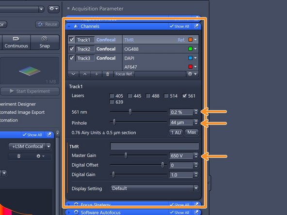
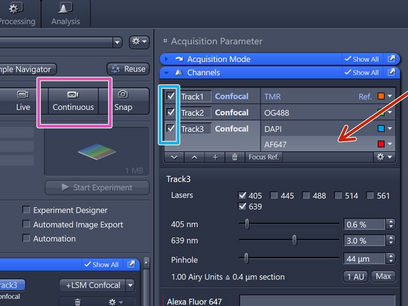
In the "Channels" box you can check which laser line has been chosen for each "Track".

In the "Channels" box you can adjust the laser power, the diameter of the confocal pinhole as well as the detector master gain.

The settings below the tracks correspond to the track highlighted in light grey.

Optimal performance of the detectors is achieved when using a master gain of 650-850V.

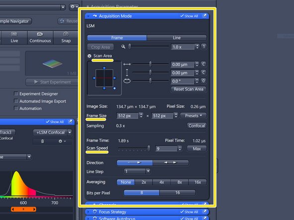
In the "Acquisition Mode" box you can change the scan area, adjust the scan speed as well as optimize the image size for optimal sampling and therefore image resolution.

More detailed explanations on the aforementioned tabs will follow in the next steps.

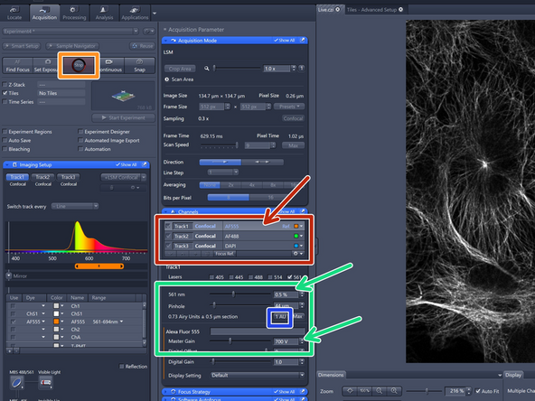
Select a "Track" for adjusting in the "Channels" box by just clicking on it. It becomes highlighted.

Click "Live" for starting the acquisition. ("Live" = fast live, always 512x512 format)

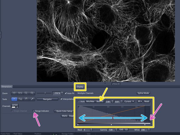
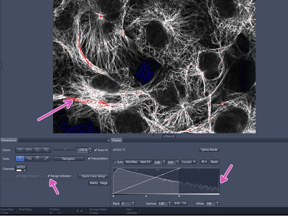
Adjust the "Display" histogram by clicking "Best Fit" for seeing an image.

Refocus by using the hardware focus wheels or by holding "Ctrl" and using the mouse wheel.

Adjust pinhole to one airy unit by simply clicking "1 AU".

Optimize the image quality by adjusting the detector gain as well as the laser power.

Fill the histogram to ensure usage of full dynamic range while avoiding any saturation of your image.

Check the histogram (peak at the highest grey level) and/or tick the "Range Indicator" (red pixels) to check for saturation. Peak/red pixels should be omitted.

This short video briefly summarizes the previous step.

Be sure to always fine-tune your focus so you are optimizing to the brightest image plane. Double check your finalized settings by focusing through your samples, making sure no plane shows any saturation.

Repeat for the other set up "Tracks".

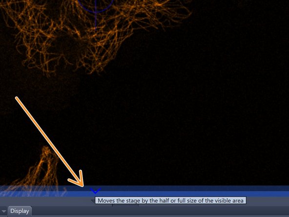
You can adjust position while live scanning within the software:

Simply double-click on the desired area in the live image and this particular positions gets centered.

Click at the outer edges moves the stage in that direction.

Proper setting of the xy sampling (pixel size) is crucial for acquiring optimal images.

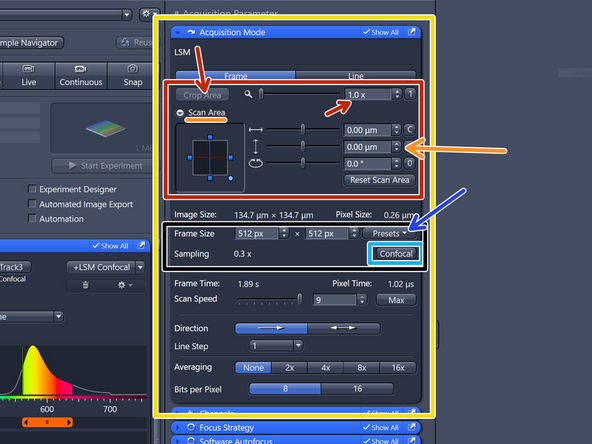
Open the "Acquisition Mode" box.

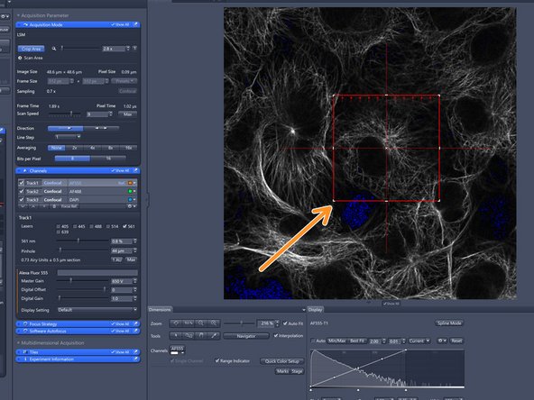
Change your field of view by using either the zoom factor (the area of interest should be centered) or choosing "Crop Area".

Interactive Crop: Place, rotate and adapt the crop area according to your needs on the live image. Or simply manually enter values in the scan area section.

"Frame Size" defines the number of pixels in one scan area.

Click "Confocal" to optimize pixel size according Nyquist criteria sampling (gets highlighted if active - if active it automatically adapts the pixel size according to the zoom).

To adjust for the correct pixel size you can further use the online calculator such as the SVI Nyquist Calculator and adapt the pixel size manually via the "Preset" Formats or simply typing values in.

Increases acquisition time if large field of view.

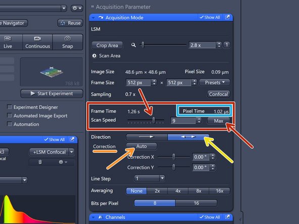
Change the "Scan Speed" by adjusting the slider or clicking "Max" (always uses fastest possible scan speed independent of changing zoom or frame size) (highlighted if active).

Use slower scan speeds to increase the pixel dwell time and thus collect more light.

You can also activate bi-directional scanning to speed up acquisition.

Please make sure it is properly aligned. Otherwise press the "Auto" button.

When using bi-directional scanning, speed higher than 9 should not be chosen to guarantee for proper alignment over the whole field of view.

When faster scanning speeds are required the multiplexing mode (MPLX) using the airy detector is recommended. For this please refer to the dedicated guide.

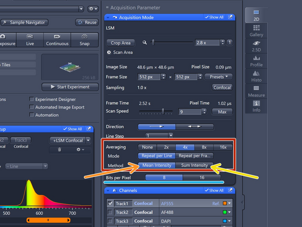
If you are limited by the laser power but still need to increase the signal ( or reduce noise) use "Averaging":

"Mean Intensity" ("Repeat per Line or per Frame"): may be used to remove noise (e.g. if high gain is used).

"Sum Intensity" ("Repeat per Line or per Frame"): useful for very weak signals.

If applied acquisition time will increase.

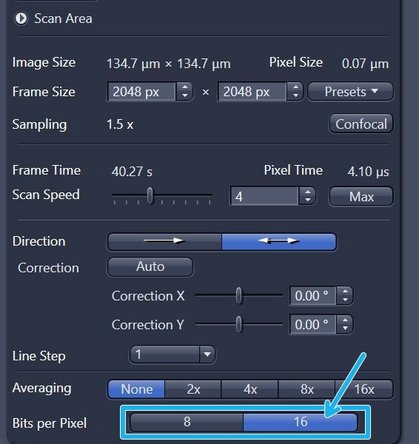
Set "bits per pixel" (bit-depth) to 16 bit. This will ensure that our dynamic range is sampled as widely as possible.

''Bits per pixel: Ideally you want to set this value to match the analog to digital conversion being done by the LSM hardware. Converted into a 20-bit space.

Select another "Track" in the "Channels" box to adjust those settings. Repeat for all available "Tracks".

"Live" = fast live, runs always in 512 x 512 format, max speed, and displays only the "Track" highlighted in light grey.

You can switch between "Tracks" while being "Live".

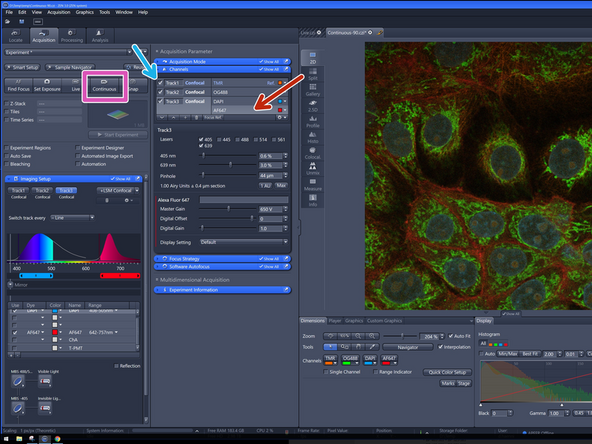
Finally press "Stop" and click "Continuous" for a live view of all channels as well as using the resolution as defined in the "Acquisition Mode" box.

"Continuous" runs the live scan in the experimental settings (chosen format, pixel size, speed e.g.)

The checkbox indicates which tracks are scanned in continuous mode.

If adjustment is necessary, untick the other tracks for ease of use and faster scanning.

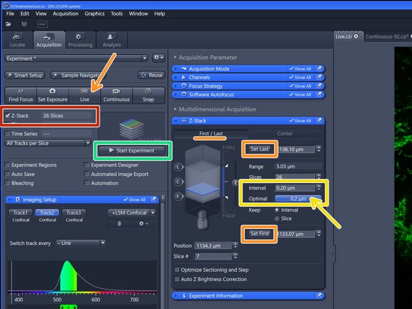
Activate the "Z-Stack" checkmark.

Press "Live" and focus through your sample to set/adjust the z-stack boundaries ("Set First" and "Set Last") in the "Z-Stack" menu box.

Click "Optimal" in the "Z-Stack" menu box for automatically optimizing the z sampling ("Interval" = z-step size).

You should refer to the SVI Nyquist Calculator if you plan to deconvolve your image as a post-processing step.

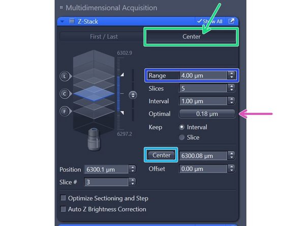
Alternatively you can define your Z-stack by setting your focal plane / center of your Z-stack. Click on "Center" option.

Set your focal plane by manually focusing and click "Center".

Set your "Range" (3D-Volume) which should be acquired.

"Center" is the matter of choice if z-stacking is combined with "Tiles regions" or "Tiles positions" (please refer to the appropriate guide).

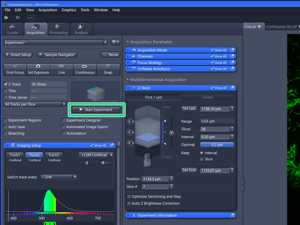
Click "Start Experiment" for acquiring the defined "Z-stack".

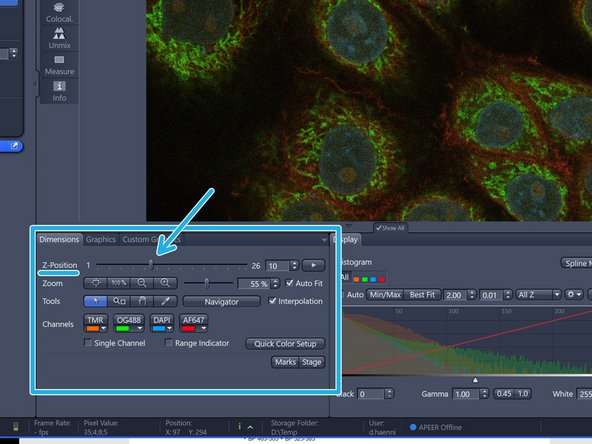
After acquisition you can navigate trough the slices of your stack in the "Dimensions" tab.