Introduction
Principle of Structured Illumination Microscopy (SIM)
Structured Illumination Microscopy (SIM) uses a sinusoidal pattern to enhance image resolution. This pattern can be a 1D line grid (Stripe SIM) or a 2D dot pattern (Lattice SIM), with defined periodicity. The pattern is positioned in the excitation path, conjugated to the image plane, and projected onto the image, modulating the excitation intensity along the pattern. This modulation also affects the fluorescence, with the highest contrast in the focal plane. The contrast decreases with distance from the focal plane, but depth discrimination in the axial direction is possible due to the Talbot effect. The grid constant ideally matches the cut-off frequency of the system. Interferences from diffraction orders generated by the grid enable lateral and axial light structuring.
Key Concepts
Pattern Projection and Modulation:
- The sinusoidal pattern is placed in the excitation path, conjugated to the image plane, modulating the excitation intensity and resulting in a modulation of fluorescence.
- The highest modulation contrast is in the focal plane, decreasing with distance, enabling axial depth discrimination through the Talbot effect.
Grid Constant and Diffraction Orders
- The grid constant ideally equals the cut-off frequency of the system.
- Interferences from the diffraction orders are used for lateral and axial light structuring.
- For optimal resolution enhancement, the grid constant should be smaller than half the wavelength, allowing a two-fold enhancement in both lateral and axial directions.
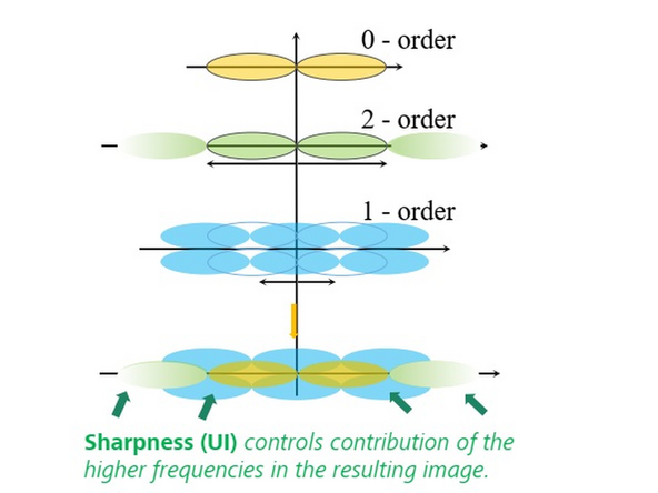
Interference Orders:
- A coherent image generated with a sinusoidal line grid pattern involves three interference orders:
- 0th Order: From the 0th order non-diffracted beam.
- 1st Order: From interferences of the 1st order diffraction beams with the 0th order non-diffracted beam, shifted by half the modulation frequency.
- 2nd Order: From the interference between the +1st and -1st order diffracted beams, shifted by the modulation frequency, containing high-frequency information for resolution enhancement in X and Y.
- The 1st order contains information for sectioning and better z-resolution.
Pattern Generation and Image Reconstruction:
- The pattern generated with a linear grid involves three-beam interference.
- In 2D Lattice SIM, the pattern is generated by a five-beam interference, resulting in seven orders.
- Since resolution is only obtained in the orientation of the grid pattern, typically three rotations are used for a line grid pattern, requiring a minimum of 15 images (3 rotations x 5 phase shifts each).
- In Lattice SIM, due to the symmetrical pattern, no rotation is necessary, but a minimum of 13 phase-shifted images (2 x 7 orders - 1) are required.
- A final back transformation from the frequency space to the real space generates the high-resolution image.fluorescence microscopy.
-
-
Differences to previous versions
-
SIM processing in ZEN Black SR 3.0 was CPU based. Therefore it was quite slow.
-
3.10 is now using GPU-accelerated SIM processing.
-
For GPU parallel processing to work, the algorithm had to be switched from the “Fourier” space into the image space.
-
It is therefore a totally new algorithm that was implemented for GPU-acceleration
-
Change of the settings and defaults
-
-
-
Widefield images: Any 2D image contains z plane information + out-offocus information from all other sections.
-
Missing cone in Z ~ lack of resolution
-
“Extending the resolution, in a true sense, is equivalent to finding a way to detect the information from outside the observable region” Gustaffson 2008
-
Reconstruction assumes that the 3D data include the entire emitting object → need all the data for order combination and a model of the PSF
-
WF deconvolution constraints: non-negativity of the density of the fluorescent dye
-
-
-
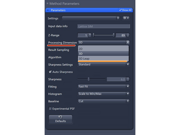
Processing Dimension: select 2D, 2D+, 3D or 3D Leap (auto for Leap data)
-
2D+: similar to Airyscan 2D (Jost et al), processing algorithm will use the PSF (experimental or theoretical) to deconvolve and get a pseudo 3D stack, getting better 2D
-
3D Leap: only for Leap datasets
-
-
-
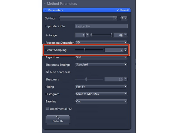
Results Sampling: sampling of the final image (pixel size) but also the available frequency space to reconstruct the higher resolution information.
-
Result Sampling 1: Maintains the pixel size of raw image in the output image.
-
Result Sampling 2: Halves the pixel size of raw image in the output image (Nyquist sampling for max SIM resolution).
-
Result Sampling 3: Splits the pixel size of raw image into thirds in the output image.
-
Result Sampling 4: Quarters the pixel size of raw image in the output image (Nyquist sampling for max SIM² resolution).
-
For both SIM Apotome and SIM² Apotome, the improvements in resolution typically do not justify any oversampling.
-
For Lattice SIM and Lattice SIM² reconstruction: if the signal-to-noise ratio (SNR) is very high, the pixel size of the rendering may become a limiting factor, necessitating an increase in sampling.
-
-
-
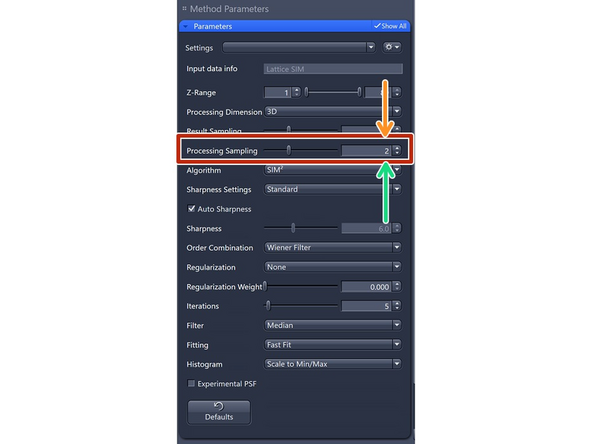
''Only available if SIM² as "Algorithm" is selected.' as this oversampling is required for the iterative SIM processing.
-
Processing Sampling: oversampling of the pixels in the raw data, getting finer pixels and data. Oversampling of 2 increases the file size by factor 4.
-
For SIM Apotome, resolution improvements do not necessitate oversampling, key is speed and sectioning → keep at 1 (Maintains pixel size of raw image).
-
For Lattice SIM, start with 2 for weak signal (halves the puxel size of raw image)
-
3 for good SNR (splits the pixel size of the raw image into thirds)
-
4 for extremely good samples and structures at the resolution limit. Quaters the pixel size of the raw image.
-
-
-
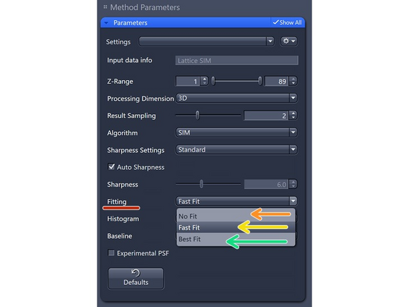
Fitting: try to determine the parameters of the excitation (pattern grating and phases) peaks of the different orders in Fourier space.
-
Fast Fit (default): This method selects a subset of the raw data that shows the most contrast to perform the fitting and determine the phases and orders.
-
Estimates parameters for the whole image.
-
Best Fit: This method is suitable only for good signal-to-noise ratio (SNR) data. It is more time-intensive as it splits the image into tiles for detailed analysis and parameter determination. This approach is effective when dealing with areas susceptible to aberrations, such as interfaces and refractive index (RI) jumps.
-
Estimates parameters for quadrants of the image.
-
No Fit: Use this method only if the Best Fit method doesn't work and for very sparse samples, such as in DNA-FISH.
-
Takes theoretical parameters.
-
-
-
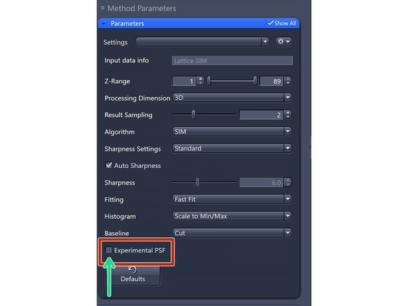
Experimental PSF: The point spread functions (PSFs), or more accurately, the optical transfer functions (OTFs) of the system will be used in the order weighting for image reconstruction.
-
Note: You can use the ZEN PSF Wizard to model refractive index mismatches. Theoretical PSF is often more robust, as users frequently make mistakes in PSF measurements and generation, which can lead to significant errors.
-
We reccomend using the theoretical PSF so do not check this box.
-
-
-
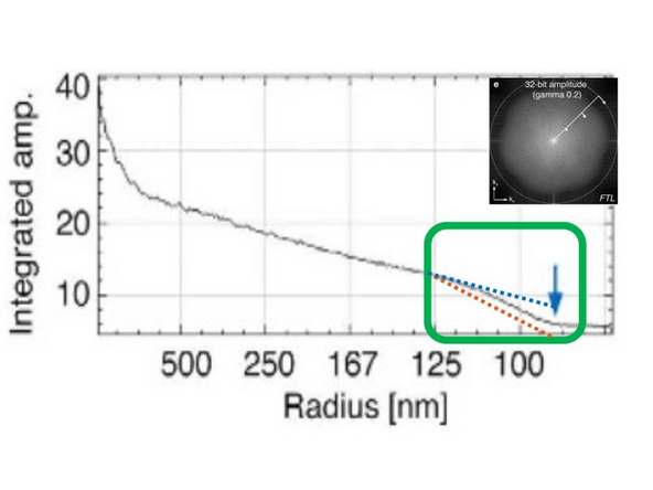
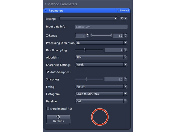
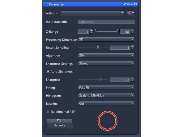
Sharpness Settings: Auto, with 3 empirical settings for the automatic Wiener reconstruction based on the raw data’s signal-to-noise ratio (SNR) and frequency content. These settings will vary depending on image quality and will assign a value to either maintain, boost, or dampen the higher frequency range (see curve).
-
Standard (default): Defines the amount of contribution from higher frequencies.
-
Weak: Reduces the contribution of higher frequencies.
-
Strong: Increases the contribution of higher frequencies.
-
Manual: Lower numbers dampen higher frequencies; values over 10 strongly enhance them. Decrease sharpness by 1 unit from the auto-value if *artifacts appear. Increase by 1 unit if higher frequencies or resolution are needed.
-
*Artifacts such as ringing around structures or negative dips appear.
-
-
-
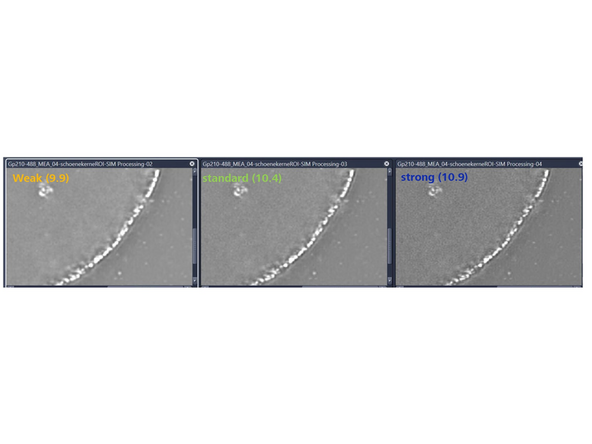
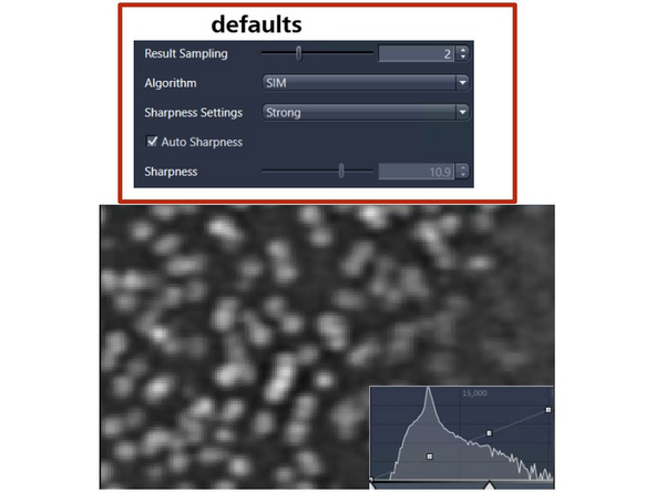
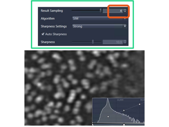
Image reconstruction – effect of results sampling & sharpenss
-
Here an example of GP210 (nuclear pore complex - seen as rings).
-
It appears we are limited by the pixel size in the result, as some substructure is still visible. The pixel size is 30 nm.
-
Increase the "Result Sampling" or decrease the pixel size to 20 nm, and you will start to separate the structures a bit better.
-
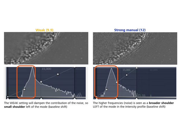
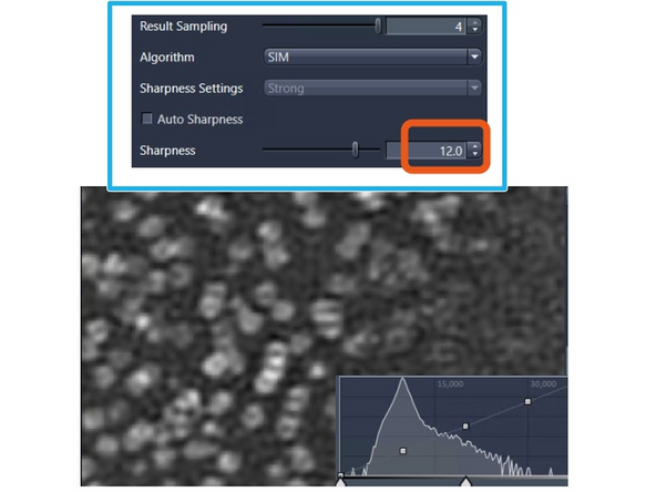
Increase the "Sharpness" to include more higher frequency and resolution information.
-
This will make the nuclear pore rings visible but also introduce more noise artifacts (e.g., shoulder in intensity profile). To mitigate this, you would want to attenuate slightly (regularize).
-
-
-
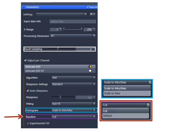
Histogram: How to scale the intensity histogram after the reconstruction.
-
Scale to Min/Max : Scales the histogram range to the maximum dynamic range.
-
Scale to raw: Keeps histogramm range from the raw image (use if TILING).
-
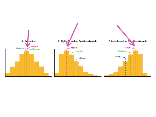
Baseline: How to render the intensity histogram after reconstruction.
-
Cut: This will remove the negative values, resulting in some pixel values being set to 0.
-
Shift: This will shift the entire histogram. For rendering, place the minimum display slider at the mode.
-
This enables the evaluation of the contribution of noise and higher frequencies
-
What is mode of an histogram?
-
-
-
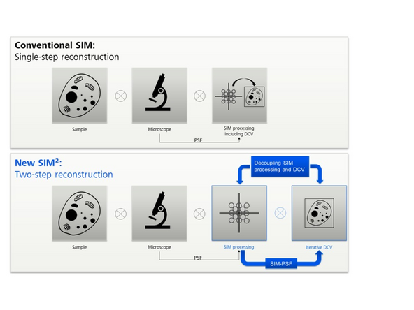
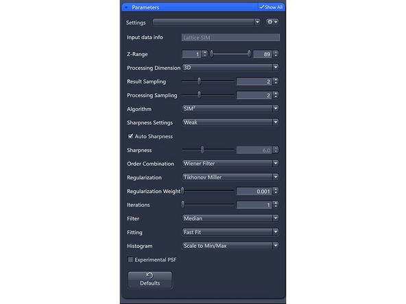
SIM² is a two-step reconstrution procedure.
-
At the first step, separated orders are combined by weighted summation.
-
At the second step, a Richardson-Lucy deconvolution algorithm with some *regularization/constraints is applied.
-
Regularization can help manage noise and ensure that the reconstructed image remains realistic and consistent with prior knowledge of the structure.
-
The PSF for the iterative deconvolution is generated in the same way as it is used in image reconstruction, by processing a point response (PSF) with the exact same parameters extracted from the data (SIM-PSF).
-
As with any iterative deconvolution, there are many possible "solutions." The key is to find the one that is closest to the underlying structure.
-
Similar to other iterative deconvolution software packages, ZEISS added "regularizers," which utilize pre-existing ("a priori" ) knowledge of our structure to limit the solution space. These regularizers generally help remove "noise" or "roughness" at the edges of the Fourier image.
-
Common priors include smoothness, sparseness, sparse gradients, non-local priors, and many others. These regularizers limit the space in which we search for our reconstructed image solution.
-
-
-
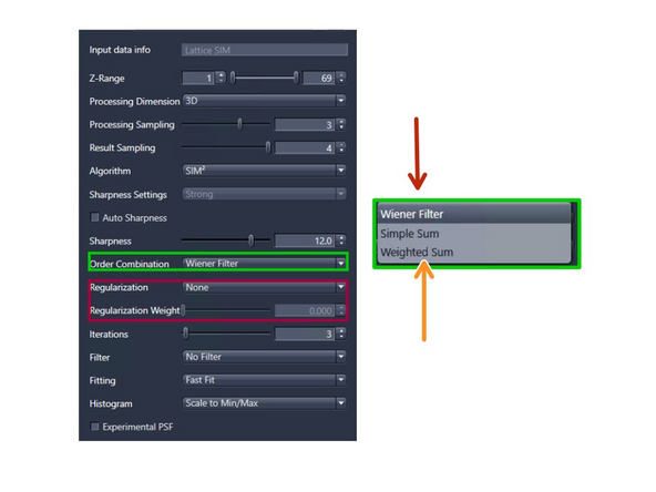
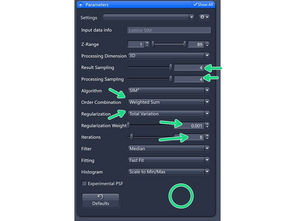
Order Combination: Scales how orders are summed up.
-
Wiener Filter (default): Sums up the orders by Wiener filtering. Most robust for noisy data – will not get rid of the noise totally
-
Frequency Dependent Weights: The weights applied by the Wiener filter depend on the frequency.
-
Overlap Impact: Where orders overlap, the filter will have a stronger impact.
-
Sharpness Parameter (Auto): The sharpness parameter is automatically adjusted.
-
Weighted SUM : Uses sum with somewhat over-weighted higher orders. For high SNR datasets.
-
Order Strength Proportional Weights: The weights are proportional to the strengths of the orders and are consistent for the entire order.
-
Optimal for High SNR: This method is ideal for data with really good signal-to-noise ratio (SNR).
-
-
-
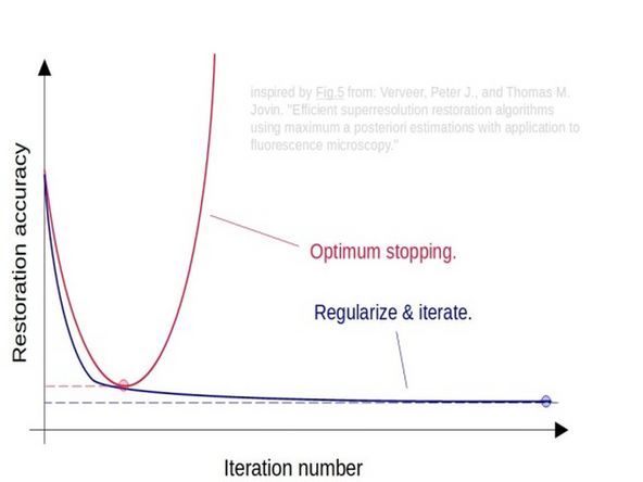
Deconvolution and SIM processing can be performed using various algorithms such as the Richardson-Lucy algorithm, Wiener filter, and maximum likelihood estimation. These algorithms use different assumptions and regularization techniques to estimate the original signal from the convolved or degraded version.
-
Since deconvolution and SIM processing are ill-posed problems, meaning there can be multiple possible solutions for the same degraded signal, regularization is used to limit the solution space and obtain a unique and stable solution.
-
Interestingly, early stopping acts as a highly efficient regularizer! Rather than applying regularization and running many iterations, it often makes sense to simply stop the restoration at the optimal point. However, finding this optimal point is the tricky part.
-
-
-
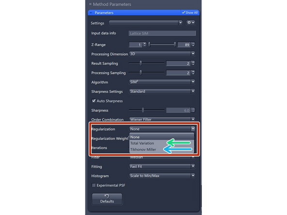
The regularization parameter balances how well the model fits the acquired data and how much regularization is applied. Increasing this parameter adds more regularization, which helps prevent the model from overfitting the data.
-
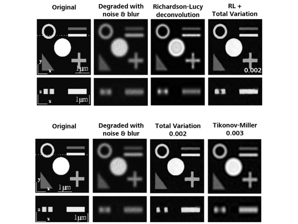
Total Variation: Better at separating spots. Start with 0.001, increments of 0.001 – max 0.004.
-
Measures Differences: Calculates the sum of absolute differences between adjacent pixels for the entire image.
-
Minimizes Fluctuations: Aims to minimize the total variation of the image, ensuring that intensities do not fluctuate too much.
-
Reduces Noise: Helps reduce noise and smooth the image without losing details.
-
Tikhonov-Miller: Better at Smoothing (e.g., DAPI). Start with 0.001, increments of 0.001 – max 0.004.
-
Compute Differences: Calculates the difference between the reconstruction and the original image.
-
Noise Reduction: The regularization term enforces noise reduction, resulting in smoother and more regular solutions.
-
-
-
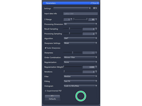
Low intensity / Live imaging / Diffracting tissue
-
SIM recommendations
-
SIM² recommendations
-
-
-
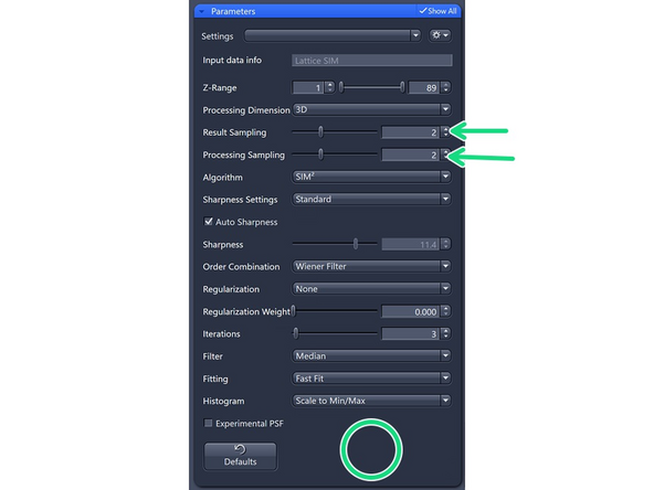
Live/tissue, diffracting but big signal amplitude.
-
SIM recommendations
-
SIM² recommendations
-
-
-
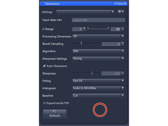
e.g. close to coverslip, fixed neurons
-
SIM recommendations
-
SIM² recommendations
-
-
-
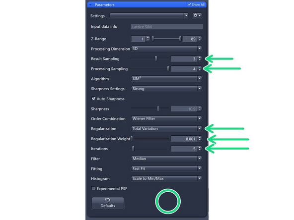
nuclear pores, fixed mito, actin
-
SIM recommendations
-
SIM² recommendations
-
-
-
Not for users that are interested in nuclear organisation!
-