Leica SP8 inverse (Schlieren) - Part 2: Adjusting excitation and emission settings

Click button "Switch to Classic UI"

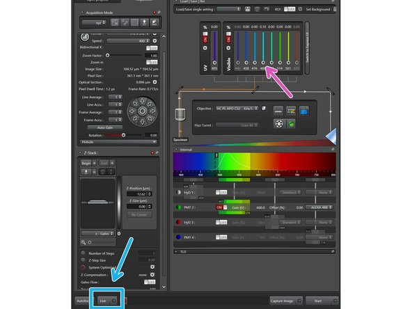
Activate UV and/or visible lasers by clicking the buttons.

Increase the laser power to a low percentage value like 0.1%. You can control the laser power by

pushing the intensity slider directly,

via the mouse wheel (after clicked once on the white dot),

or by simply entering a value (double-click the displayed intensity value).

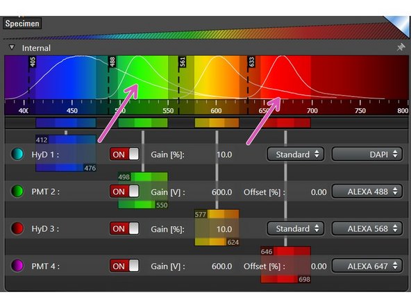
You should see a laser line in the emission spectra settings once you activated laser power.

The SP8 is equipped with two types of detectors.

PMT (Photomultiplier Tubes).

PMTs have a larger dynamic range than HyDs and tolerate high signal saturation.

HyD (GaAsP Hybrid Detectors)

HyDs are more sensitive and show less noise compared to PMTs. However, they are more fragile and you must not record strongly saturated signals. HyDs can further record in "photon counting mode" which can be useful for quantitative analysis.

Press buttons to turn on individual detectors.

Once a detector is activated you can select an emission spectra from the drop down list. This is very handy to evaluate potential crosstalk between dyes and to set the detection range.

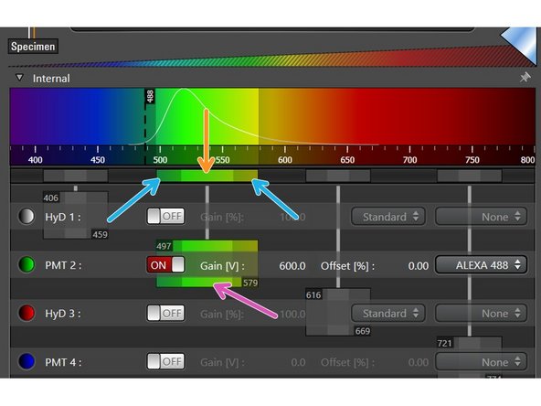
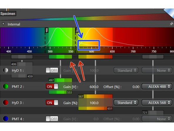
The detection range of each detector has to be defined individually for the corresponding dye. Take the displayed emission spectra as help.

Click in the middle of the detection window (left mouse button ), and drag the detection range under the emission curve.

Pressing and dragging the dark colored edges (left mouse button) lets you change the size of the detection range.

Alternatively, you can double-click the detection range to enter values directly.

Ensure that the minimum distance between detection range and excitation laser line is at least 6 nm, to avoid unwanted reflections.

While positioning your detection windows also consider potential spillover.

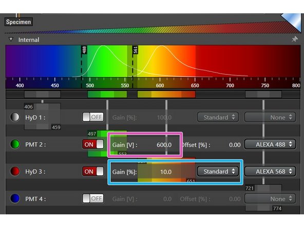
For PMTs gain adjustment is necessary (between 600V to 900V usually generates satisfying results).

For HyDs you can also select a gain when working in Standard mode. Try to reduce the gain to 10% when having sufficient signal intensities for optimal results

You can adjust the gain of the detector by double-clicking the numerical value to enter the value directly or moving the corresponding slider.

The default gain for PMTs is set to 0 (you won't see anything if not changing) and for HyDs it is 100% (strong gain which may emphasize noise signal).

Start adjusting the first channel by:

Click "Live" button

Increase laser power until you get an optimal illumination of your sample (see next step for tools to verify this).

If you cannot observe any signal in your image even with high laser power...

double check the detector gain setting

is there any light coming out of the objective when running the live mode? If not change to the "Configuration" tab and check the laser settings.

switch back to widefield mode and confirm the sample is in focus

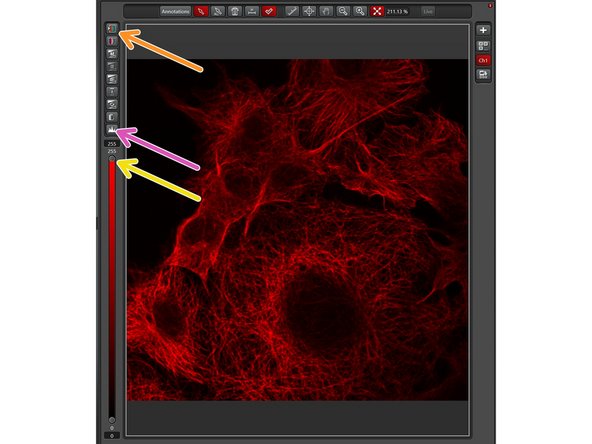
To aid the adjustment of intensities in the image, click on the LUT icon to choose the "glow-over-under" lookup table. In this display mode, pixels with maximal intensity are shown in blue while pixels with 0 intensities are shown in green.

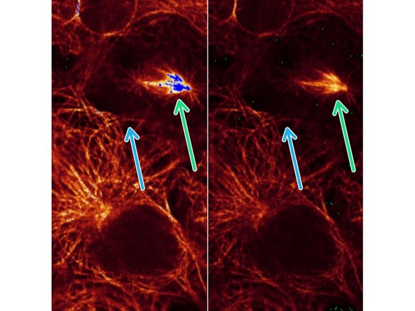
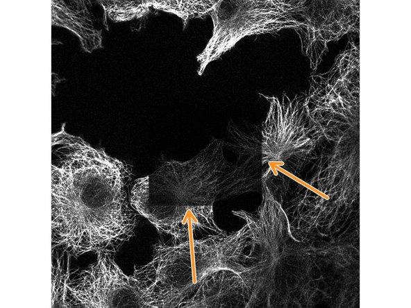
Example of microtubule staining recorded with different laser power

Here, the mitotic spindle is getting saturated on the left (blue pixels) while reducing laser power prevents this on the right image.

However, neighbouring cells show less well resolved microtubule structures after reduction of laser power.

In most cases, it makes sense to adjust the signal intensities for the structures of interest. Exceptions may be quantitative signal measurements of the total image.

Activating the image histogram is an alternative approach to identify saturation and may help to evaluate signal to noise ratio. Generally, try to avoid under- and overexposure.

For weak signals it is useful to adjust the display properties by moving the slider down.

Repeat step 5 and step 6 until you have set up all channels of your recording.

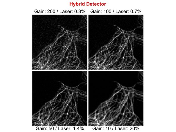
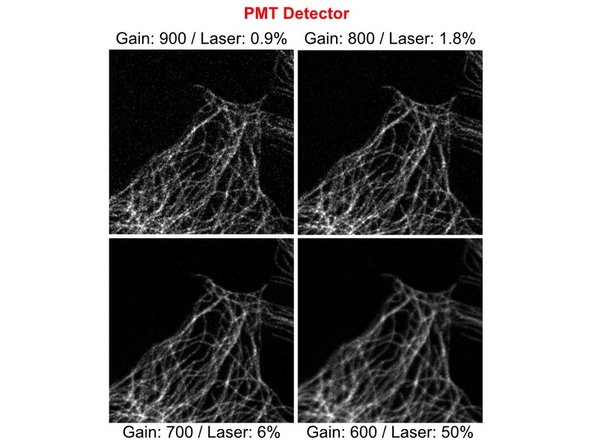
The same image of a cellular microtubule network was recorded with different detector gain settings. Laser power was adjusted to result in comparable signal intensities for all images.

Note how signal to noise ratio improves from top to bottom right with lower Gain settings and higher Laser Power.

Hybrid detectors often generate a slightly better signal amplification than PMTs and then provide a better signal to noise ratio with lower laser power settings.

Prolonged laser scanning at high intensity resulted in signal bleaching at the imaged region. Bleaching can be noticed e.g. by decreasing signal intensities during a z-stack scan or like in this example after reducing the zoom factor.

For each experiment you will need to find the optimal settings for detector gain and laser power. Try to keep the detector gain at low levels for best signal to noise but increase it if you notice signs of bleaching!

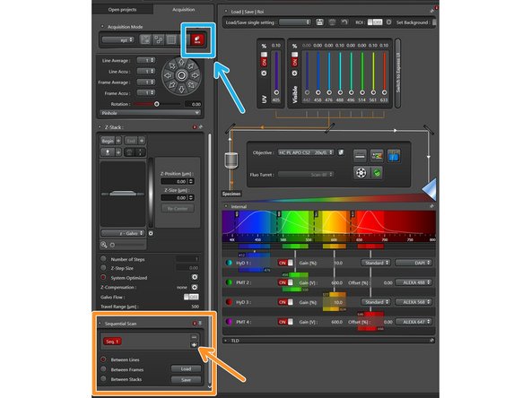
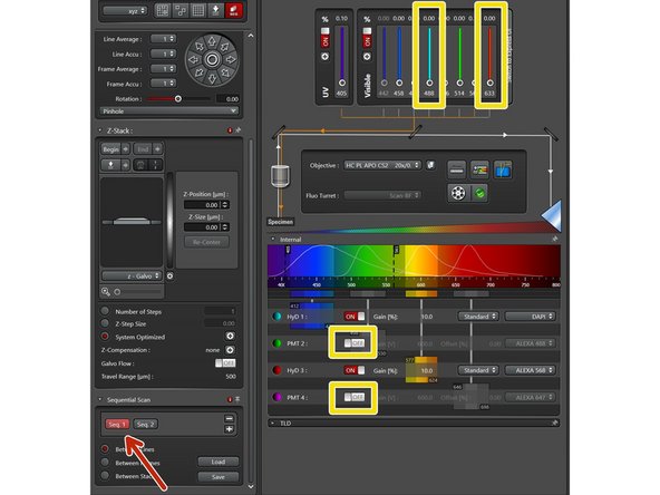
Some emission curves are very broad and it may be impossible to avoid spillover into other detection channels (DAPI is a typical example for this). In this case you will need to perform sequential scanning.

Click on the icon for sequential recording.

The sequential scan menu will appear and you can add additional sequences by clicking the plus symbol.

Click on the sequence you want to edit.

Switch off laser power and detectors for the channels you do not want to record in this sequence.

Change to next sequence and repeat procedure for channels which were not selected yet.

You may also record all 4 channels in this example sequentially. This would be necessary if all the emission spectra have some overlapping regions. However, this would significantly increase the scan time because each sequence will be recorded independently. We recommend to combine channels whenever possible!

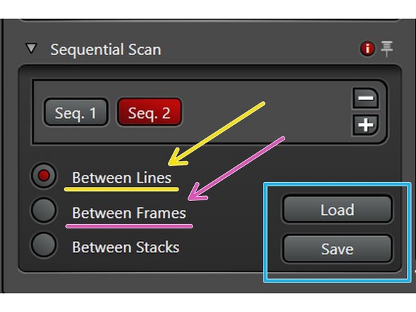
Scanning modes:

"Between Lines" for faster acquisition (only laser lines will change but detection windows must stay the identical between sequences).

"Between Frames" for more flexibility (if detection windows should vary between sequences, and/or different accumulations/averaging settings are applied).

The "Between Frames" mode even allows to use the same detectors for different sequences.

You can Load/Save the excitation, detector and emission spectra settings via these buttons.