Introduction
This guide of the Center for Microscopy and Image Analysis explains how to count nuclei in HCS images acquired with the HCS - MD ImageXpress Confocal HT.ai and export the results.
NOTE 1: It is made for single-timepoint, multi-site, and multi-well acquisition for one channel (DAPI). Please adapt it to your own needs if you have different acquisition settings.
Note 2: Think beforehand how to design your plate. The data will be sorted by well A1-A12, B1-B12 etc.
-
-
Start the "MetaXpress" software either on Special VM B or on the dedicated Special MetaXpress VM.
-
Login with the same name and password as on the machine.
-
-
-
Go to "Screening" and select "Review Plate Data [DB]".
-
In the "Review Plate Data" window, click "Select Plate" to choose your plate to be analyzed.
-
Your plates are first ordered according to the acquisition date. Double-click to open the folder.
-
The different plates acquired on that day will appear below.
-
"Select" will open the respective plate data.
-
-
-
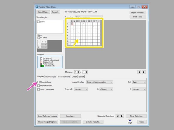
The plate format shows up. "-" indicates that these wells were imaged.
-
If you have run an analysis on this plate before, you can hide the values (Low Pressure) by unclicking "Show values" in the "Display tab".
-
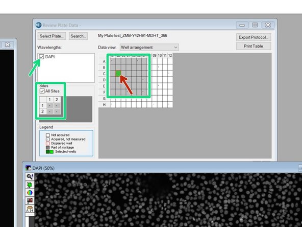
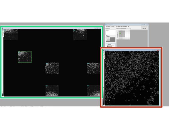
For a montage, mark the corresponding wells, define the sites per well and select a channel for display.
-
For a high-resolution image of one site in a well, right-click on the corresponding well.
-
Please note that by right-click you will also automatically mark the cell for analysis.
-
-
-
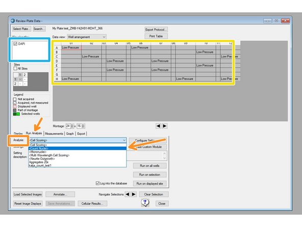
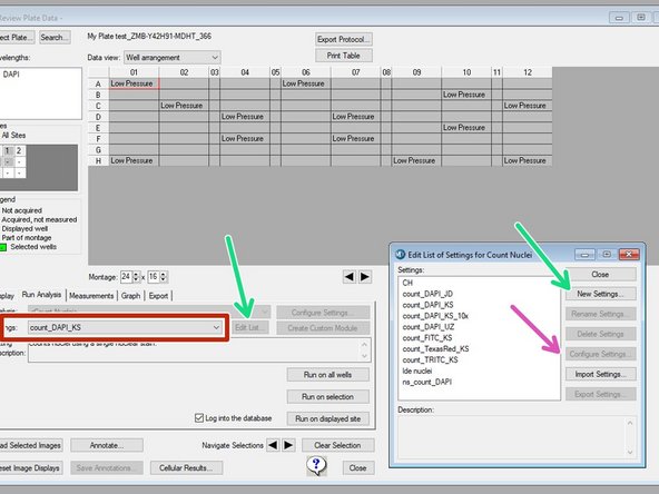
In this example, a previous analysis has been performed on the plate.
-
Select your channel to be displayed and analyzed.
-
In the "Run Analysis" tab, under "Analysis" select "<Count Nuclei>".
-
If you already have saved settings, you may proceed to the next step.
-
Please do not overwrite other users settings!
-
To create your own settings, click on "Edit List" and "New Settings" with your specification.
-
Click on "Configure Settings" to adjust the segmentation parameters.
-
-
-
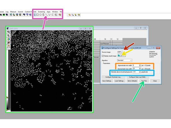
Choose your channel for the segmentation: "DAPI".
-
Choose how to display the results (we recommend "New").
-
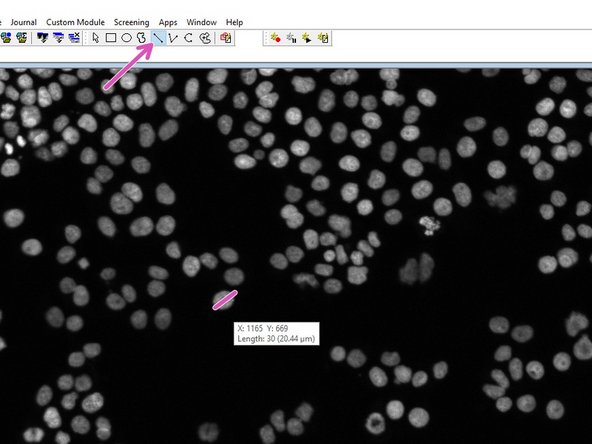
In the drawing toolbar, choose "Line" to measure the width of a few nuclei by clicking on one end of the cell and by placing the mouse over the diameter and getting the distance.
-
Measure a few cells and use these values for the "Approximate min./max. width" for segmentation.
-
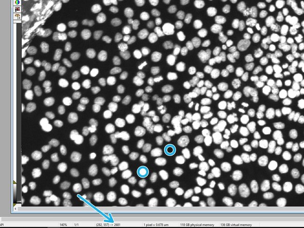
Hover over regions of cells and background and check the intensity in order to choose the segmentation parameter "Intensity above local background".
-
Click "Test Run" to test the input settings.
-
-
-
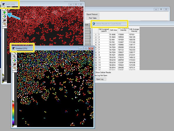
When the analysis is done for your test image, an overlay of the segmentation will be shown in red together with your grayscale image. Additionally, a color-coded segmentation image and cell-by-cell results will be shown.
-
Show/hide the overlay to judge the quality of the results.
-
If necessary, go back and adjust the input parameters to improve the segmentation.
-
If you are happy with the result, click "Save Settings".
-
It might be worth checking for a few images whether the input parameters work, especially when the size of the nuclei or the intensity greatly vary within your plate.
-
In order to check a different image of the same plate, go to the "Review Plate Data" tab and right-click on a different well. Do a "Test Run" again and judge the result.
-
-
-
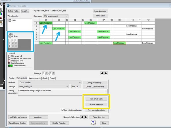
You can now run the segmentation algorithm either onthe whole plate or on on a selection.
-
If you want to run on a selection, select the corresponding wells by right-click (will appear green) and choose the sites per well.
-
If you re-run an algorithm on a plate (for the same wells), the old data can be overwritten. However, it might still be accessible for export (c.f. step 9).
-
Running the algorithm on a whole plate will take a while. When you open the plate again in the "Review Plate Data", you will see the entry "Low Pressure", which indicates that for this well an analysis has been performed.
-
-
-
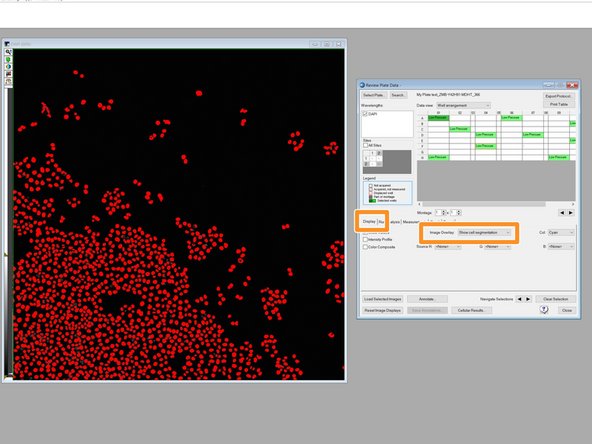
In the "Display tab", choose for "Image Overlay": "Show cell Segmentation".
-
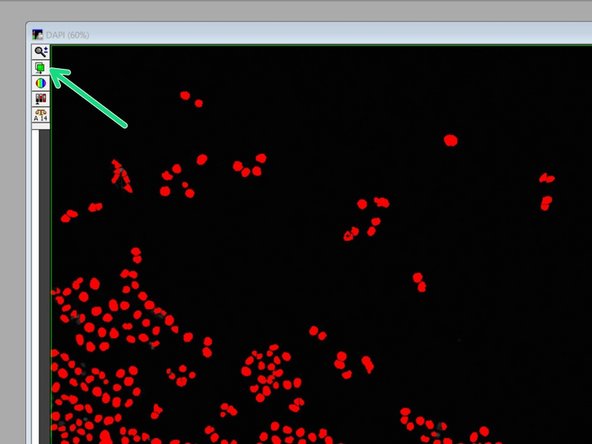
Use this button to show/hide the segmentation and judge the quality of the algorithm.
-
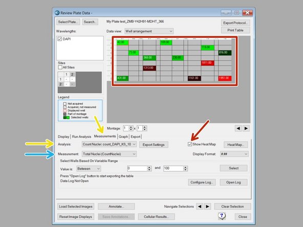
Go to the "Measurement tab" and choose the "Analysis" (if multiple were run on the same plate).
-
Choose the type of "Analysis" to be displayed.
-
E.g. "Total nuclei (CountNuclei)" gives the total number of nuclei determined by the "CountNuclei" algorithm.
-
Note: "CO2 Pressure Status" is the default, therefore "Low Pressure" as default value after analysis.
-
If you choose one site per well, the corresponding value for the site will be shown. If you choose all sites, an average (not total!) will be shown.
-
Click "Show Heat Map" to display your results as a heat map.
-
-
-
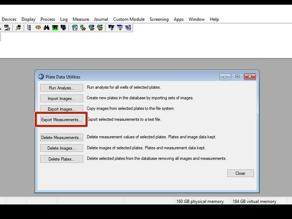
For data export, go to "Screening" and select "Plate Data Utilities [DB]".
-
Select "Export Measurements".
-
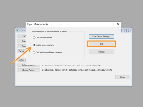
Select "Image Measurements" and click "OK".
-
"Image Measurement" will give you the measurements per image (e.g. total/average of nuclei), but will not provide information about the individual cells.
-
-
-
The measurements are first sorted according to analysis date for the plate (Measurement Set) and then for the plate (Name [Plate Info]).
-
Either double-click on the measurement or use the arrow to make it appear in the "Query" on the right.
-
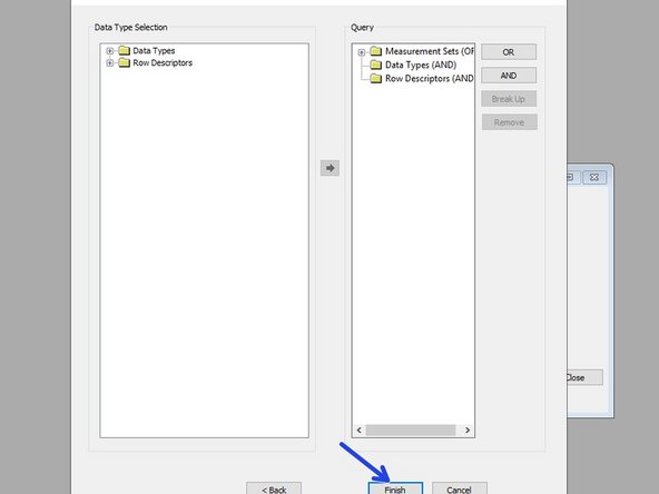
Click "Next".
-
Click "Finish".
-
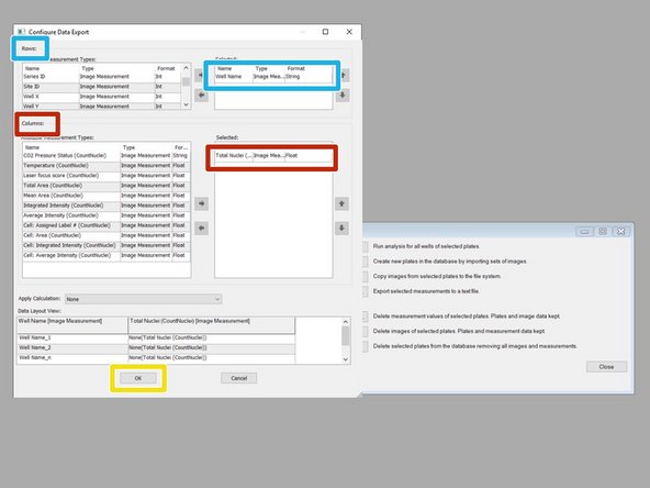
In "Rows" select "Well Name" with the Type "Image Measurement" by double-clicking so it appears on the right.
-
In "Columns" double-click on "Total Nuclei" to get the number of nuclei per image.
-
Click "OK".
-
-
-
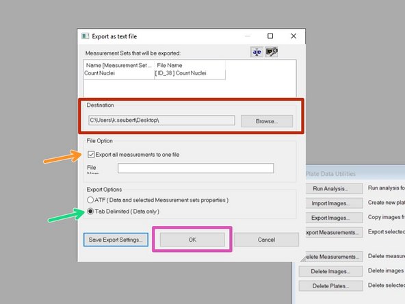
Select your export folder.
-
Check "Export all measurements to one file" and define a File Name.
-
Select "Tab Delimited (Data only)".
-
Click "OK".
-
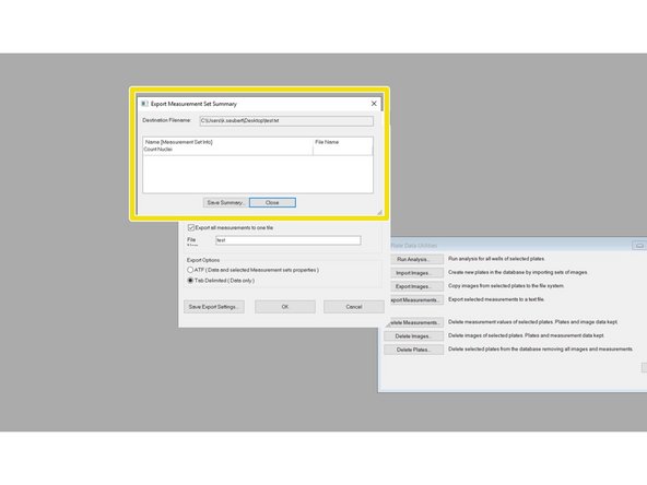
You will get a notification that the export was successful.
-
-
-
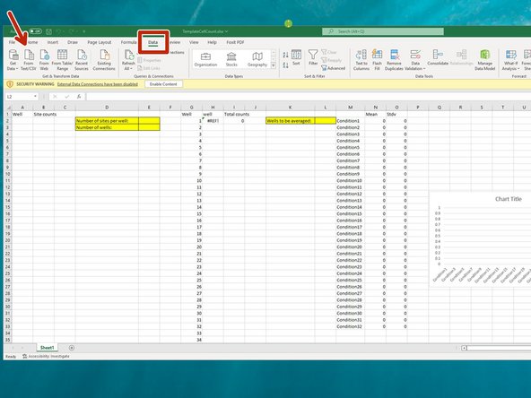
We can provide you with a basic analysis template for Excel.
-
In the "Data" tab, click "From Text/CSV".
-
Open the ".txt"-file generated in Step 9.
-
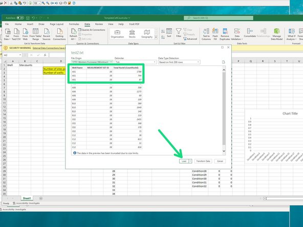
Check whether the format is correctly recognized and click "Load".
-
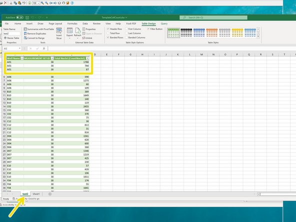
A new tab will appear with your well information and the number of detected nuclei.
-
If you have acquired multiple sites per well, the number of nuclei per site is displayed and therefore the well name listed repeatedly.
-
-
-
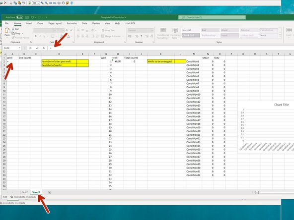
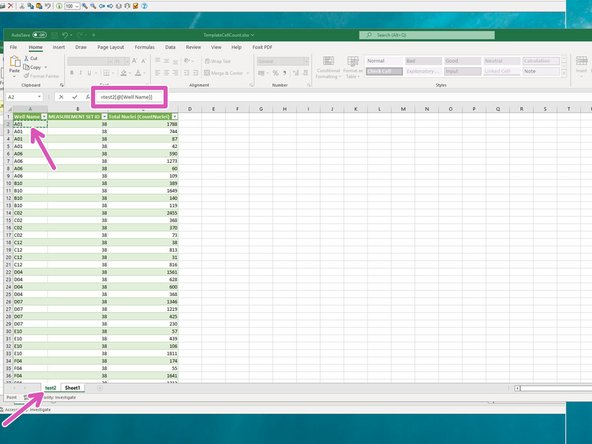
To start referencing the data, go back to the "Sheet1", click on cell "A2" and type "=".
-
Go to the data sheet (test2), and click on the first cell (A2) with a well name, with the reference appearing in the formula bar.
-
Press Enter to make the reference.
-
Repeat the same procedure for the counted nuclei by typing "=" in cell "B2" and referencing it to "C2" (Total Nuclei (CountNuclei)!) in data sheet.
-
Mark Cells "A2&B2" and extend the referencing by grabbing and dragging the lower right corner of the marked cells down to the maximum number of sites measured.
-
-
-
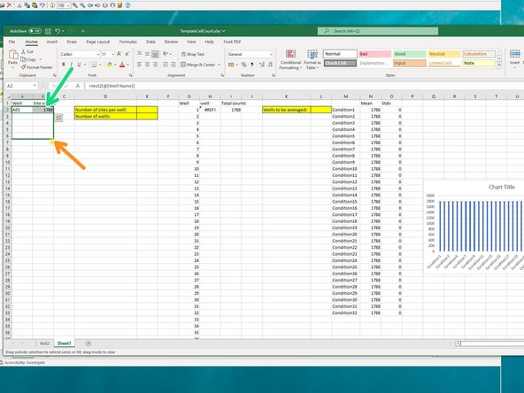
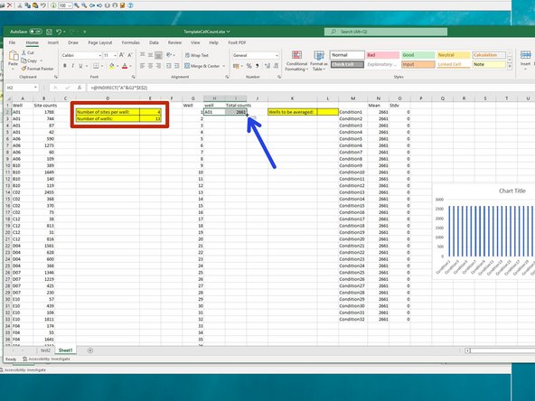
Specify the number of sites per well and number of wells.
-
This will automatically fill cells H2 and J2.
-
By grabbing the lower right corner of the two marked cells H2 and J2, drag to extend to your maximum well number.
-
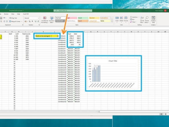
Type in the number of wells to be averaged, the corresponding mean and standard deviation will appear and the histogram will fill itself.
-
Default is average of >1 wells including standard deviation. If you want to change it, use all the tools that Excel has to offer.
-
Here you can adjust your x-axis label.
-

![Go to "Screening" and select "Review Plate Data [DB]".](https://d3t0tbmlie281e.cloudfront.net/igi/zmb/tTLYLVHVfiIb4KAU.medium)


![For data export, go to "Screening" and select "Plate Data Utilities [DB]".](https://d3t0tbmlie281e.cloudfront.net/igi/zmb/PPnLHOEBYvBr6cDS.medium)
![The measurements are first sorted according to analysis date for the plate (Measurement Set) and then for the plate (Name [Plate Info]).](https://d3t0tbmlie281e.cloudfront.net/igi/zmb/HIchopUpLqnaLTWI.medium)