Introduction
The Stellaris 5 microscope contains application-oriented imaging tools based on fluorescence lifetime which allow you to add an additional level of information to your confocal images: The Tau-Sense modes. They can help you visualize different lifetimes and also separate signals with overlapping spectra based on lifetime information.
Four different modes are available:
1) TauContrast offers a semi-quantitative method of visualizing/quantifying different lifetimes based on the average arrival time of the photons. This tool is also very handy for first inspection of your staining (e.g. to see whether it originates from an autofluorescence signal).
2) TauGating separates the signal into different images based on fixed, user-defined time gates. A useful application is to separate signal from autofluorescence (which usually has a very different lifetime).
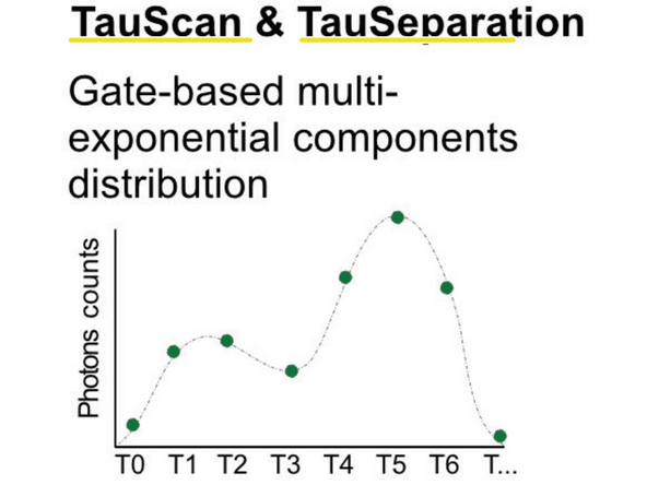
3) TauScan divides the signal into a defined number of subimages according to their lifetime. This separation includes gating and fitting. It is ideal to explore the lifetime landscape of your sample.
4) TauSeparation divides the signal into a defined number of subimages similar to TauScan. However, this separation can be fine-tuned by manually defining the populations lifetimes. Therefore, it is ideal to separate lifetimes where TauGating is not giving satisfactory results.
For more details, please read the application note "TauSense: a fluorescence lifetime-based tool set for everyday imaging", available upon request from the Leica website. Some of the illustrations were taken from this publication.
The sample cell line (microalgae Chlamydomonas exressing a cell-wall tagged mVenus additional to the present chlorophyll and extensive autofluorescence) used in the screenshots of the software was cordially provided by the Gademann lab.
-
-
For all the TauSense modes, a time-resolved photon counting is needed. The photon arrival times are recorded relative to the preceeding laser pulse of the WLL.
-
Because the 405nm laser is a continuous wave laser, the TauSense modes do not work with it.
-
Lifetime-based information adds an additional level of information to the confocal image. Structures with the same spectral properties can be distinguished based on fluorescence lifetime.
-
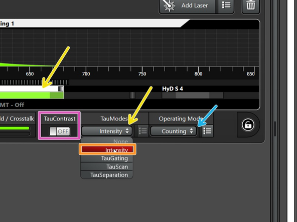
After clicking on the detector, the different "Tau modes" are visible in the drop-down menu.
-
The "TauContrast" is listed separately.
-
All TauSense modes work in the Operating Mode "Counting". So best select it from the beginning on.
-
"Intensity" is the simplest Tau mode and corresponds to the usual confocal image (loaded by default).
-
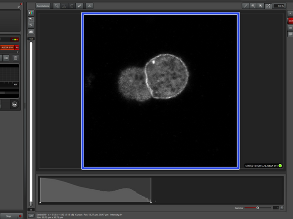
This is how an Intensity image of the sample would look like, where one cannot distinguish different structures.
-
-
-
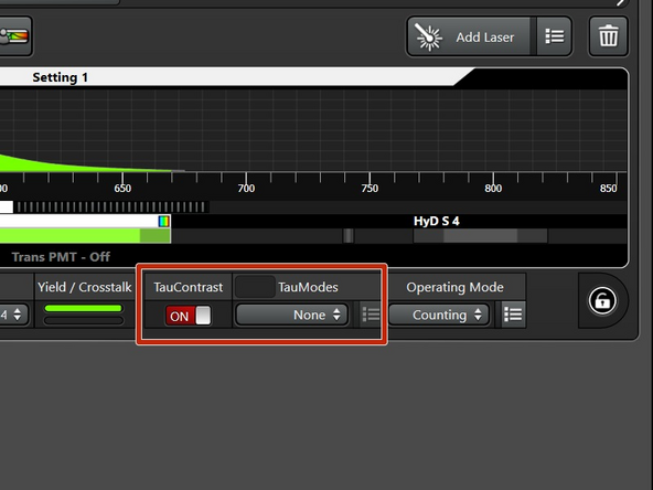
Switch on the "TauContrast" mode.
-
TauContrast produces two different images: an intensity and lifetime-image (avarage arrival time of the photons), which are overlaid in the software. In order to avoid redundant (intensity) images, you can chose "None" in the TauModes.
-
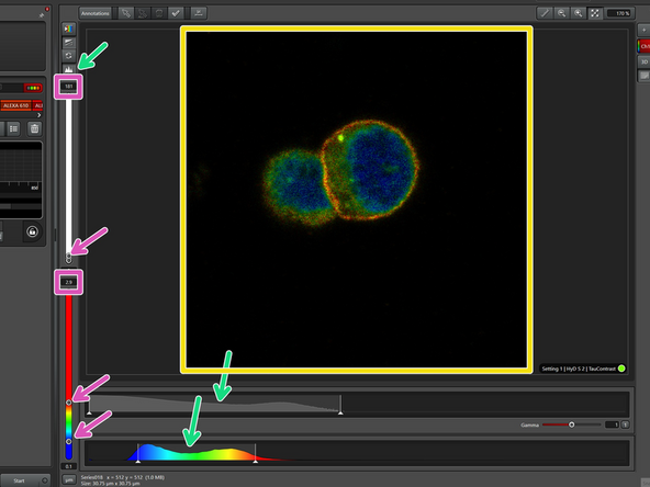
The TauContrast image contains both intensity and lifetime information
-
Because of these two layers of information, you have a histogram for both intensity (top) and lifetime (bottom).
-
To accurately display the variations in intensity and lifetime, you may need to adjust the scale either by using the slider or by entering the values manually.
-
This tool is also very handy for first inspection of your staining: If the lifetime population is at 0 ns, it is most likely autofluorescence and not an organic dye or fluorescent protein.
-
-
-
After choosing the TauMode "TauGating", click on the symbol to set the gates. These gates set a specific time window for photon arrival, and the photons that arrive within this window are used to create the image.
-
TauGating can be useful to separate clearly different lifetime signals, e.g. coming from fluorescent proteins and autofluorescence.
-
Here you can choose the number of channels (=number of images to be generated). Minimum is 1 and maximum 2.
-
If you just want your image to be "cleaned" of autofluorescence, one channel (=one image) might be perfectly enough.
-
You can set various gates within one channel.
-
All the photons detected across all the gates in a single channel are combined to produce a single intensity image.
-
The result of TauGating are 1 or 2 intensity images.
-
-
-
TauSeparation and TauScan are both based on gating combined with linear unmixing.
-
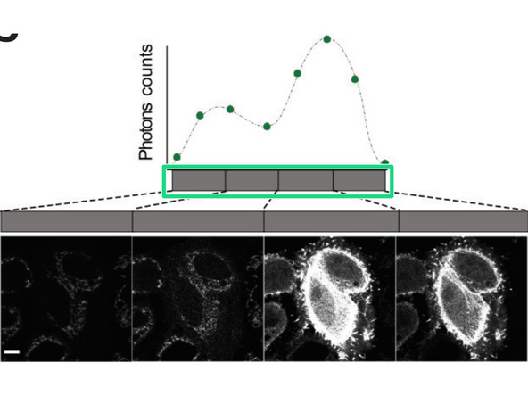
In TauScan, the software automatically sets the equally spaced gates based on the number of images to be taken. This is ideal to explore the lifetime-landscape of your sample and to detect possibly hidden lifetime populations.
-
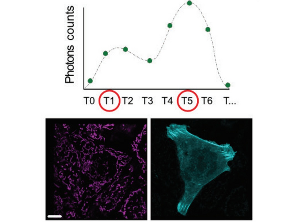
In TauSeparation, you can define the population based on the lifetime diagram.
-
In the simplest case shown here with only two populations to be separated, all photons arriving before T1 will be gated into channel1, all arriving after T5 into channel 2. All photons in between will be distributed based on linear unmixing.
-
The separation of the images is done directly at the scanhead. So there is no possibility for postprocessing to change the populations (contrary to the more complex FLIM on the Falcon).
-
-
-
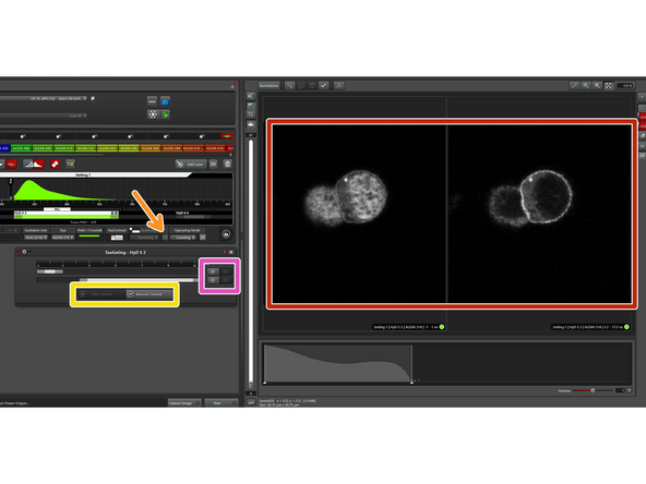
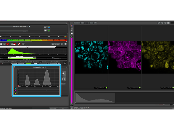
After choosing the TauMode "TauSeparation", click on the symbol to define the populations to be separated.
-
In this window, you can define how many populations you would like to separate.
-
Separation of 2 populations normally works quite well. With every additional population, the calculation gets more complicated and artifacts might accumulate.
-
For a first estimation of the best position to separate the populations, go "Live" and click on "Find".
-
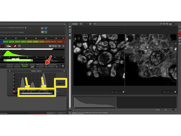
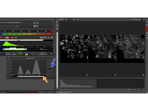
If you are not happy with the result, you can fine-tune with the sliders and see on the fly the change in the images.
-
If a third (small) population is present, you can of course also try to separate this one. In this case, it resulted in a medium quality image of some autofluorescence.
-
-
-
The TauScan mode is ideal to detect possibly hidden lifetime populations. Also here, activate the options window after choosing "TauScan".
-
You can choose the "number of images" to be separated and the software will automatically set the populations equally spaced in log scale.
-
If you increase the number of images to be separated, the lifetime range will be newly spaced.
-
You can also change the lifetime range to be screened.
-