Leica SP8: Acquire an image in xy and z

Go to "Configuration".

Select "Laser Config" and check if the necessary lasers are "ON".

The WLL allows selection of excitation wavelengths (up to 8 simultaneously) from 470 - 670 nm. For systems with a WLL it is set to 85% (only 70% for SP8 inverse STED 3X) by default.

On the "Hardware" tab:

Choose the appropriate "Bit Depth".

Check the option "Line average during Live acquisition".

Deactivate the option "Maximum integration time" to allow for photon counting mode (using HyDs).

Go to "Acquire".

Select "Laser Overview".

Set the "Frequency" to 80 MHz.

If you need the 440 nm laser, please check the appropriate guide or ask the ZMB staff.

Make sure your sample is correctly placed and focused. Check the appropriate Start-up guide for more info.

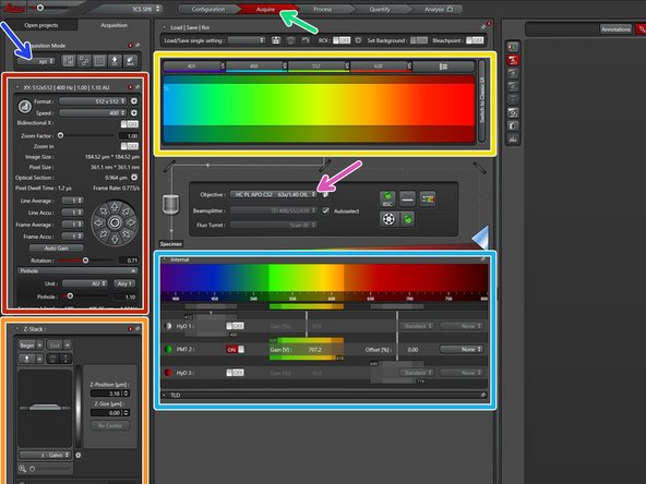
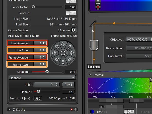
Identify the following sections in the "Acquire" panel:

Make sure you are in the "xyz" scan mode.

Settings for "XY" ("Format", "Speed" e.g. adjustments).

Settings for z ("Z-Stack" option).

Excitation settings (Laser).

Objectives.

Detectors and emission settings.

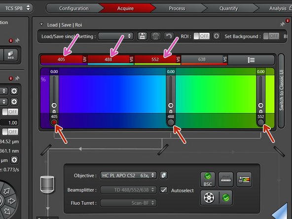
Add lasers in the beam path by clicking on the necessary lasers (if added: displayed red).

Activate corresponding UV and Visible shutters (if activated/opened: red dot).

You can control the laser power by

pushing the intensity slider directly,

via the mouse wheel (after clicked once on the white dot),

or by simply entering a value (double-click the displayed intensity value).

Once the laser is active and has power you should see an orange line indicating the light path through the objective and emission panels.

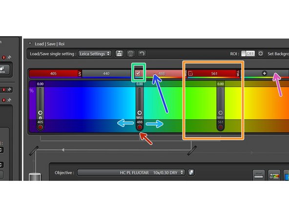
To add laser lines using the WLL use the the "+" sign.

Make sure laser lines are active (white check-mark).

If the laser is not active it will appear grayed out.

To choose the necessary wavelength you can either

drag the laser line to the correct location,

or double click the current wavelength and directly type the value in.

You can also remove unwanted laser lines by clicking on the corresponding (red) rectangle.

Make sure corresponding shutter is active (red dot).

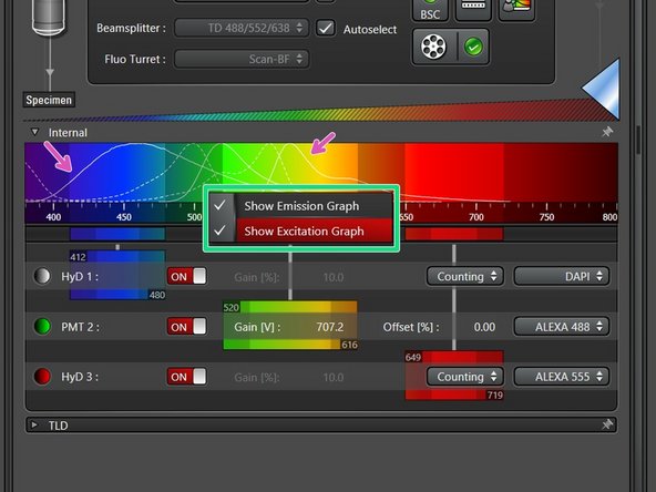
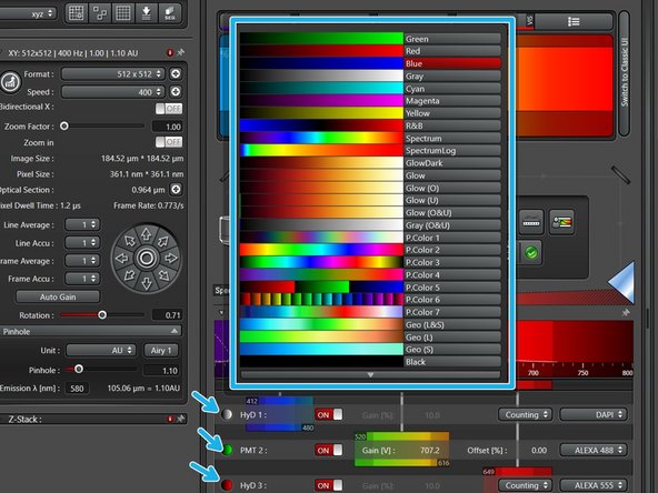
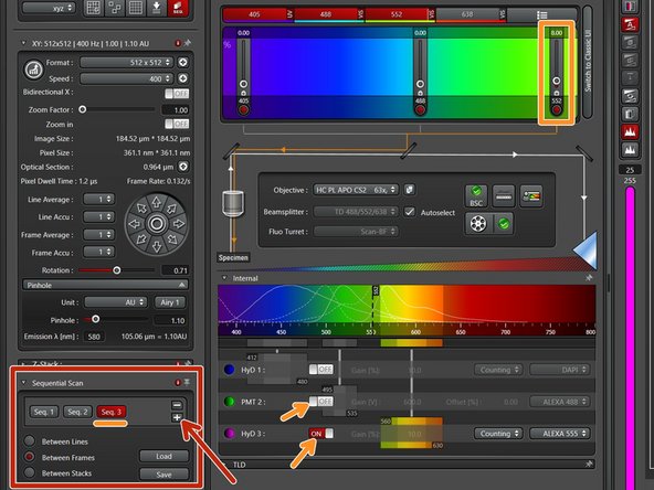
Switch "ON" desired detectors.

If applicable, set the HyDs to "counting"mode.

Here you can visualize emission- and excitation-spectra to aid placement of detectors.

use right-mouse-click into the spectrum to choose if emission and/or excitation graphs should be displayed.

Double-click on the bullets to change look-up tables (LUTs) for each channel.

This will only change the appearance of your image and can still be changed in another image processing software.

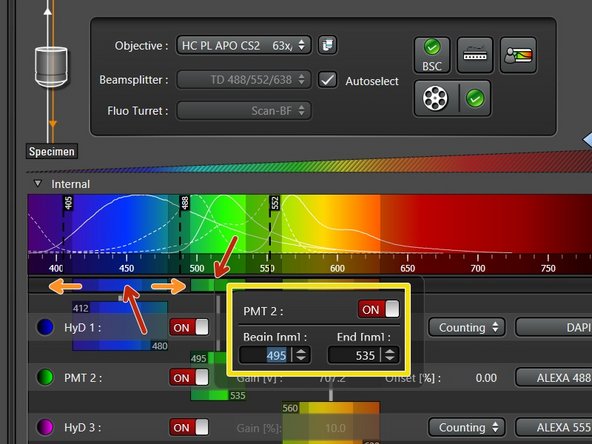
Set the desired detection range of each detector. Take the displayed emission spectra as help.

Click in the middle of the detection window (left mouse button ), and drag the detection range under the emission curve.

Pressing and dragging the dark colored edges (left mouse button) lets you change the size of the detection range.

Alternatively, you can double-click the detection range to enter values directly.

While positioning your detection windows also take care about possible bleed through.

Ensure that the minimum distance between detection range and excitation laser line is at least 6 nm, to avoid unwanted reflections.

Laser lines can be visualized in the spectrum by raising the power above 0% and making sure the shutter is opened (red dot).

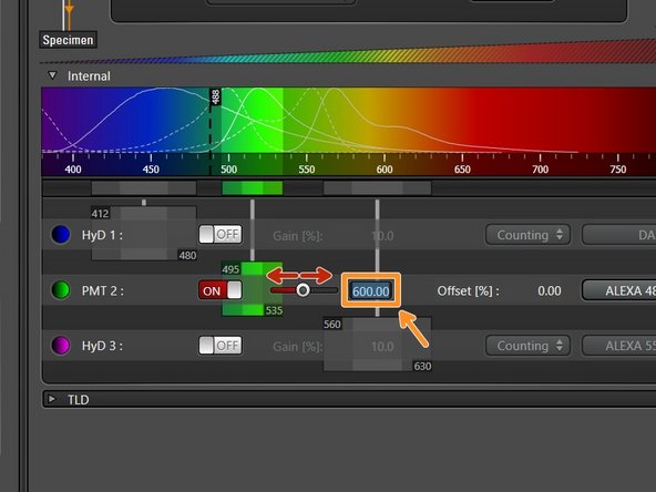
For PMTs gain adjustment is necessary (usually between 600V and 900V gives satisfactory results).

You can adjust the gain of the detector by:

Moving the corresponding slider.

Double-clicking the numerical value to enter the value directly.

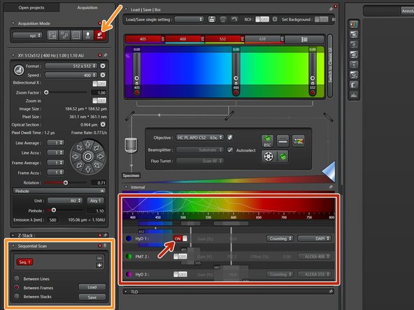
Once all detectors and lasers are set, activate only one detector and corresponding laser. Make sure all other lasers are at 0%.

Activate the "Sequential Scan" mode. A new menu will appear.

This allows definition of different sequences and thus prevents spillover between the different channels.

Select the scanning mode:

"Between Lines" for faster acquisition (only laser lines changed, detection windows must stay the same).

"Between Frames" for more flexibility (if detection windows move between sequences, and/or different accumulations/averagings are applied).

To image "in between lines" all detectors will keep positions in all the sequences. Changes made to the detector position made in one sequence will be reflected in the other sequences.

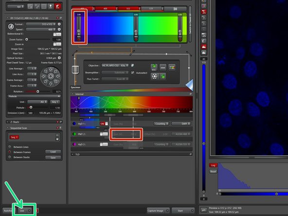
Start adjusting your first sequence.

Click "Live".

Adjust laser power.

for PMTs adjust "Gain" as described before.

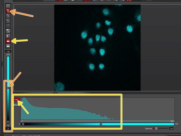
Adjust the image contrast by using the slider or activate automatic contrast adjustment ("Auto Contrast").

Activate the image histogram, click "Log" (for logarithmic display) to optimize the signal to noise ratio. Avoid under- and overexposure.

For HyD in counting mode adjust to approx. 80 counts / usec (keep an eye on the pixel dwell time - depending on the set format and scan speed). If using a PMT adjust gain and laser in a way that the histogram is filled without saturation.

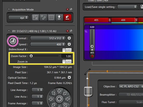
Proper setting of the xy sampling (pixel size) is crucial for acquiring optimal images.

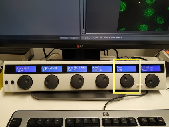
Change your field of view by using the "Zoom". You can also use the knob in the external control panel.

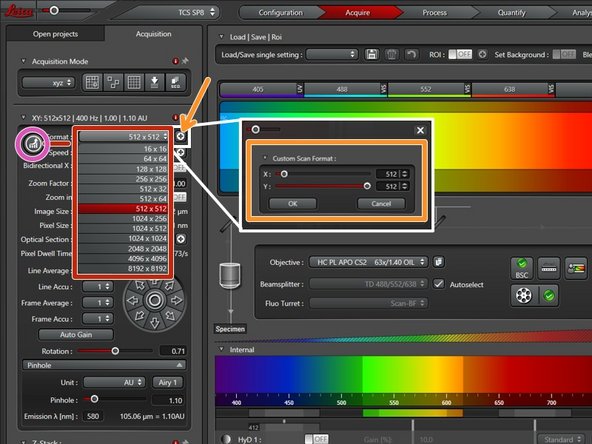
"Format" defines the number of pixels in one scan area.

One can choose preset formats via the drop down menu.

By clicking the "+" every other format can be chosen.

To adjust for the correct pixel size you can either use the online calculator such as the SVI Nyquist Calculator or the auto button for an estimate.

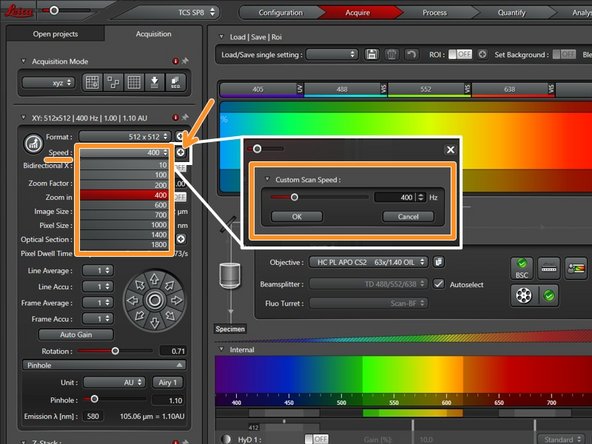
Here you can also change the scanning speed:

via the drop down menu (presets).

via "+" for every other scan speed.

Increased scan speed leads to faster imaging, lower photo-damage and bleaching, but gives more noise and allows a smaller field of view.

This option is not available if resonant scanner is used.

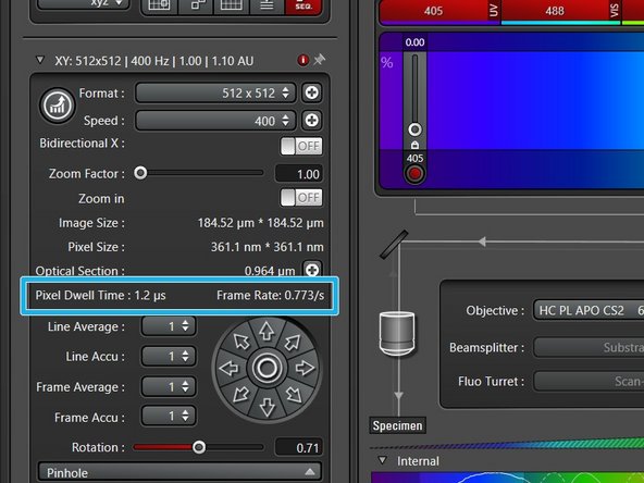
Use slower scan speeds to increase the pixel dwell time and thus collect more light.

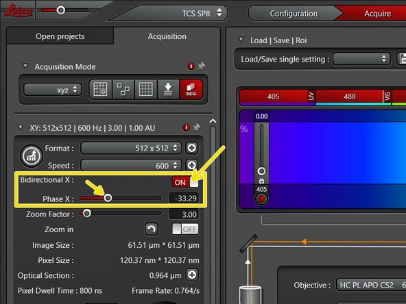
You can also activate "bi-directional" scanning to speed up acquisition.

Please make sure, the phase is properly adjusted.

If you are limited by the laser power but still need to increase the signal (or reduce noise) use:

Accumulation (by line or by frame): Useful when using HyDs in counting mode or for very weak signals.

Averaging (by line or by frame): may be used to remove noise while using a PMT (e.g. in resonant scanning).

If applied acquisition time will increase.

If more channels are necessary duplicate sequence by pressing the "+" .

Switch "ON" the appropriate detector, while switching the other one "OFF". Adjust laser powers and gain (if applicable) in the same manner.

If the fluorochromes are well separated it is possible to combine multiple fluorochromes in one sequence.

Repeat procedure if more channels are necessary.

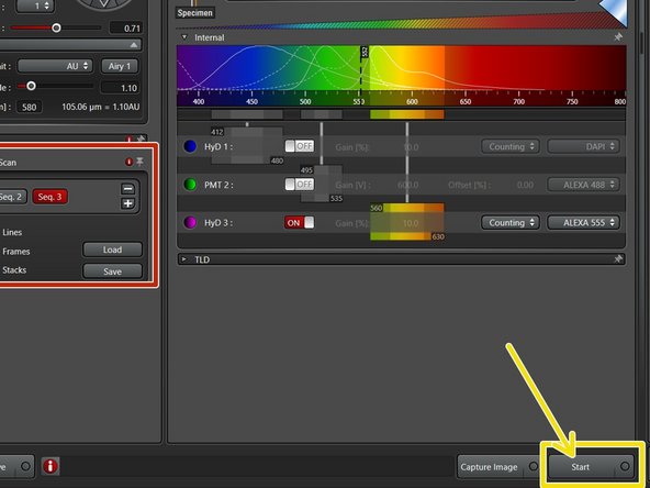
Once you are satisfied with your current settings for each seq press "Start" to acquire an image.

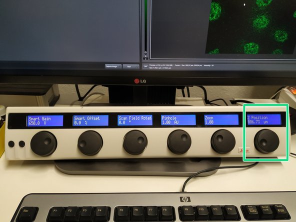
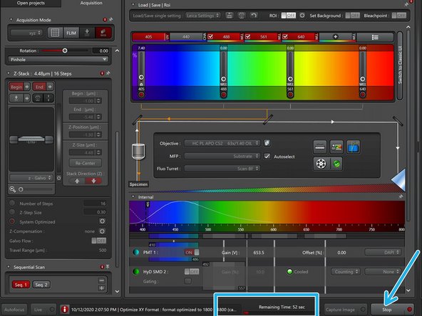
Make sure you have "xyz" scan mode selected.

Use the z-drive controller ("Z-Position") on the "control panel" to define the limits with "Begin" and the "End" of your z-stack.

Define the appropriate "Z-Step Size" or go for optimal z sampling by choosing "System Optimized". The "Number of Steps" will be automatically calculated.

You should refer to the SVI Nyquist Calculator if you plan to deconvolve your image as a post-processing step.

"Start" your experiment. The estimated time will be indicated here.

You can activate "bi-directional" scanning to speed up acquisition.