Image Deconvolution using SVI Huygens

Proper x-y-z sampling on the microscope (called Nyquist sampling) is a fundamental requirement for performing successful image deconvolution.

Out of focus information is very important for deconvolution. Therefore, it is always recommended to deconvolve 3D image datasets.

On a scanning confocal microscope you can adjust the x-y sampling by either changing the zoom or the image size and therefore changing the pixel size.

The z sampling can be adjusted by selecting the proper spacing between the slices of a 3D stack.

If you are unsure about the needed x-y pixel size and z spacing for optimal Nyquist sampling using your objective and microscope settings you can use the SVI Nyquist Calculator.

Reserve and open a ZMB image processing virtual machine.

Start Huygens Professional.

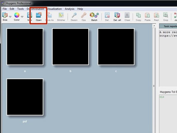
On the main menu bar click "Open".

Supported file formats include .lif (Leica), .czi (Zeiss) as well as .tif files.

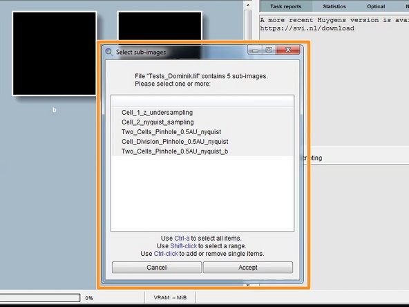
If you open a Leica .lif which can contain multiple datasets, Huygens asks you to make a selection.

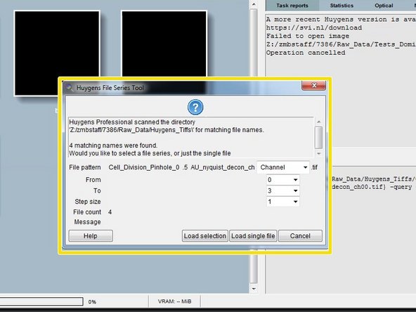
When opening a .tif series, Huygens will ask how to interpret the individual files. Such as slices from a 3D stack or time points.

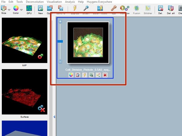
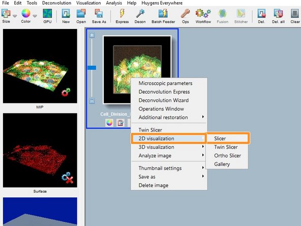
After opening a file, you should find a new thumbnail in the main work space.

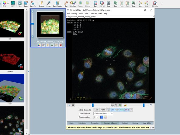
Right click on the thumbnail and "2D visualization/Slicer" opens the image in a slicer view and allows you to check if the data was imported properly.

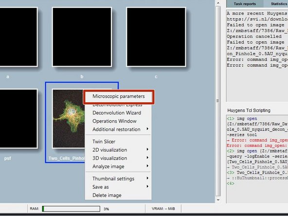
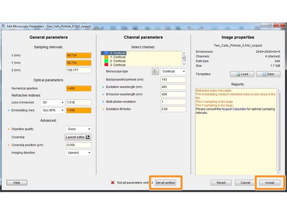
For a good deconvolution, correct microscope, image and sample parameters are very important.

Right click on your image thumbnail and select "Microscopic parameters".

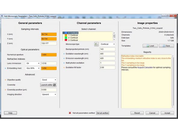
Parameters are read from the image metadata.

Depending on the source file format this parameters might or might not be correct. Check and correct them very carefully.

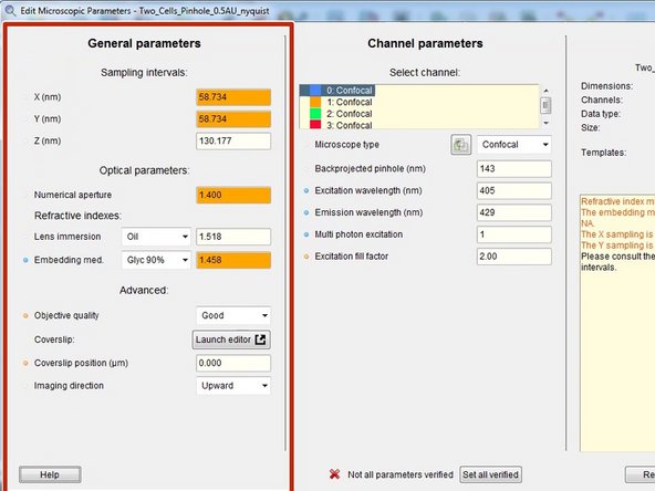
Here you can check and set the general imaging settings.

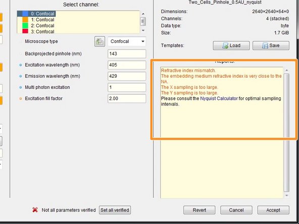
By the background color and in the "Reports" field, Huygens gives you feedback about issues with your imaging settings or parameters.

The refractive index of your sample/embedding media is only known to you and therefore has to always be set correctly.

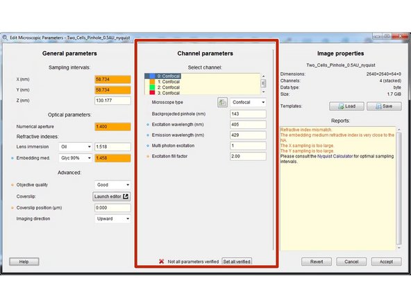
Specify the microscope type as well as the excitation and emission wavelength for each acquired channel.

For a bandpass emission filter you can use the center wavelength.

For multiphoton images you can select "Widefield" and set the "Multi photon excitation" to 2.

For standard microscopes the "Excitation fill factor" is at least 2 or higher.

For confocal microscope data the "Backprojected pinhole (nm)" is usually calculated correctly from the metadata. More information here.

For spinning disk data you can find more details here.

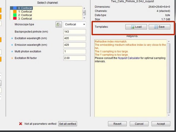
If you acquired multiple datasets with the same parameters, you can save them as a template for further use or batch processing.

After careful revision of all your parameters you can click "Set all verified" followed by "Accept".

Your data is parametrized and ready for deconvolution.

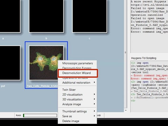
Right click on the image thumbnail and click "Deconvolution Wizard".

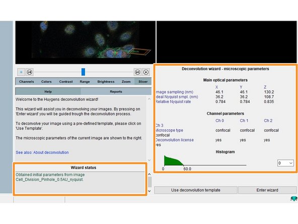
You can see some of the previously defined parameters as well as warnings about your sampling in the "Wizard status" field.

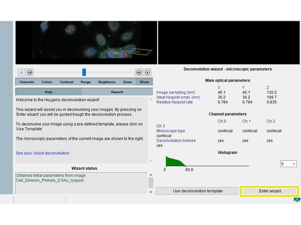
Click "Enter wizard".

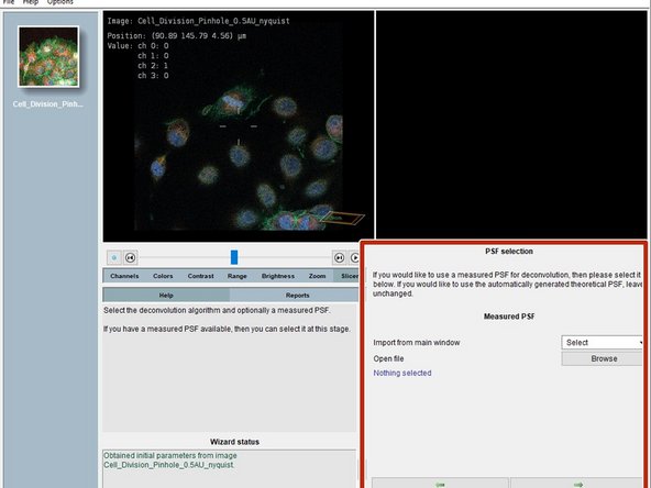
In this step you could select a measured point spread function (PSF). Usually we recommend to use a calculated one.

To automatically calculate the PSF from your parameters just click next.

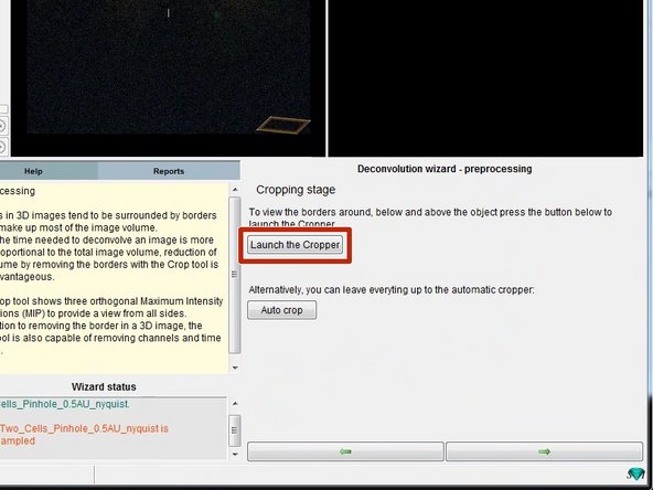
Deconvolution is a computationally expensive operation and can take quite a bit of time. In order to reduce the amount of data increasing the speed, you can crop your dataset to an area of interest.

You can crop the 3D stack by clicking "Launch the Cropper".

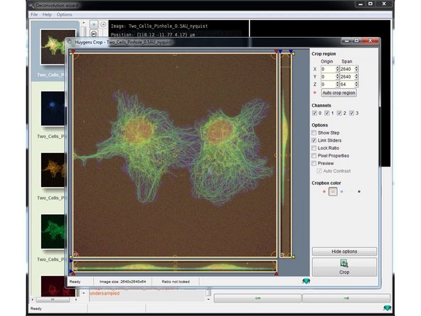
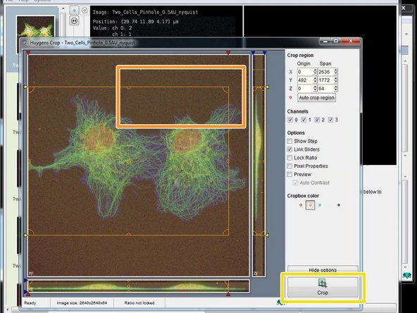
Adjust the area of interest by adjusting the cropping lines.

Click "Crop" when you are done .

Press next.

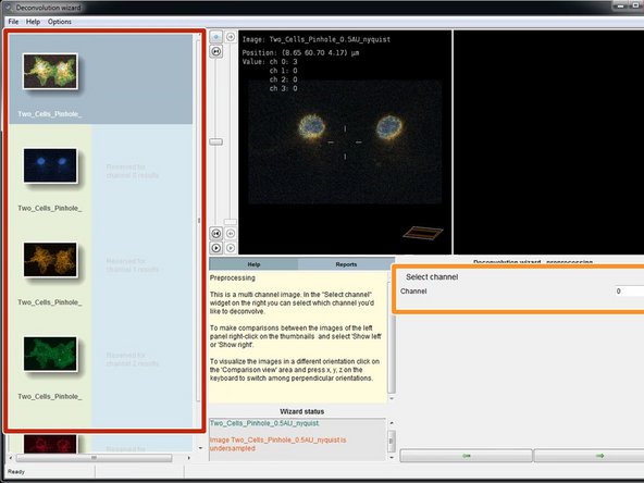
If you have more than one channel in your dataset, you will need to deconvolve them sequentially.

You can see all the channels of your dataset in the left column.

Select the first channel in the "Channel" selection and press next.

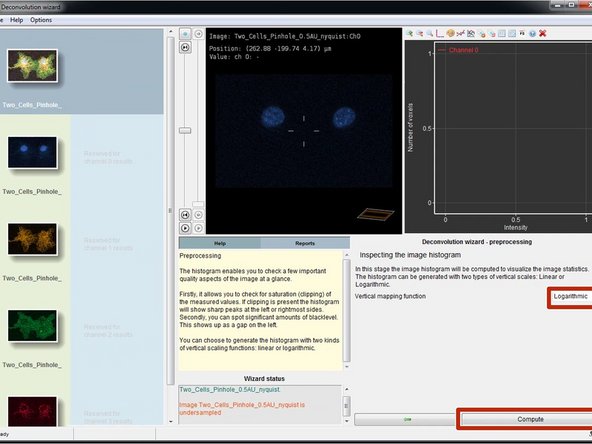
In this step you will calculate and inspect the image intensity histogram of the selected channel.

Select "Logarithmic" and click "Compute".

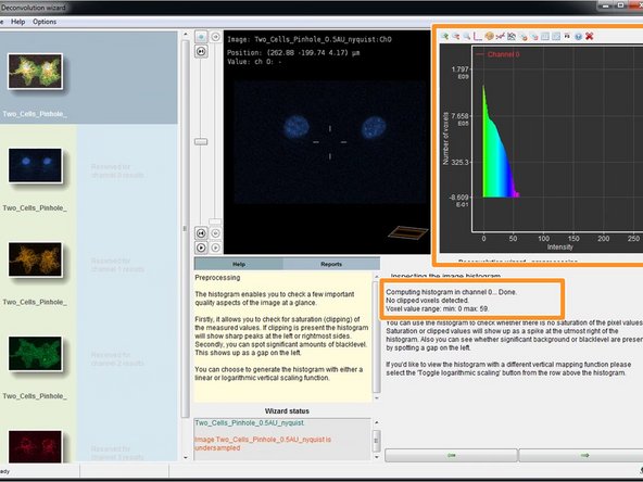
Huygens will compute and show the histogram as well as give information about the intensity distribution, such as the number of clipped/saturated voxels.

If you have clipped voxels (saturated pixels) you can still proceed with the deconvolution. However, good image statistic without clipping is important for a successful deconvolution. We strongly recommend to carefully consider this during your next image acquisition.

Press next.

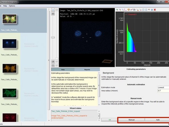
Background is any additive and approximately constant signal in your image that is not coming from the objects you are interested in. Background includes e.g. an electronic offset in your detector, or indirect light.

For low noise detectors such as the photon counting hybrid detectors (HyD) on Leica confocal systems, select "Manual" and put it to 0.

Alternatively Huygens can also automatically estimate the background based on a circular search area. For this press ("Auto").

Background removal changes the total image intensity during deconvolution. This can be problematic for quantitative fluorescence experiments.

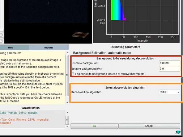
If you used automatic background estimation you can see the results in this step.

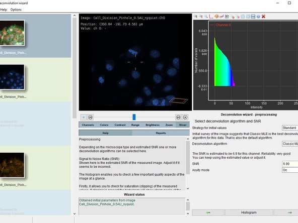
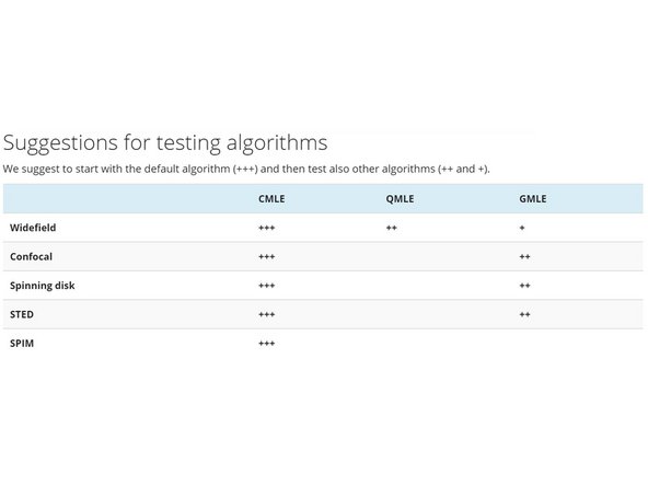
Here you can also choose between different deconvolution algorithms.

CMLE (Classic Maximum Likelihood Estimation) is the most general restoration method available, valid for almost any kind of images. It uses significantly less memory than GMLE. Usually the method of choice.

GMLE (Good's roughness Maximum Likelihood Estimation algorithm): Gives faster results (less iterations) with very noisy data such as low light confocal and STED. But uses a lot of memory.

QMLE (Quick Maximum Likelihood Estimation) is a deconvolution algorithm that gives good and fast deconvolution results on low-noise widefield images. (Not available when you deconvolve confocal images)

Check the background estimate, select the deconvolution algorithm and press "Accept".

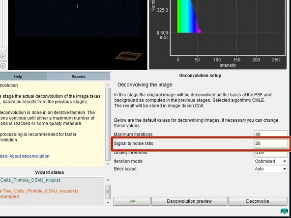
The "Signal to noise ratio" (SNR) controls the sharpness of the restoration result. The higher this value, the sharper your restored image will be. It is the most important parameter for deconvolution.

However using a too large SNR value might be risky when restoring noisy originals, because you could be just enhancing noise.

A noise-free widefield image usually has SNR values higher than 50.

A noisy confocal image can have values between 15-20.

In the Huygens Software the SNR of a digital image is defined as the square root of the number of photons in the brightest part of the image.

If you use a confocal with photon counting detectors (e.g. Leica HyDs in photon counting mode), the SNR is the square root of the highest pixel intensity in your image.

Also check the SVI Huygens webpage for further information about the SNR.

The remaining options usually don`t need any adjustments.

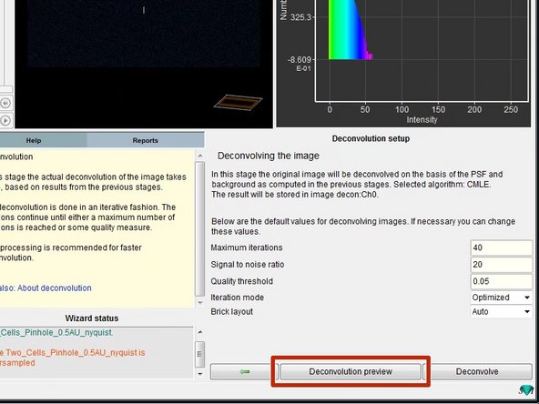
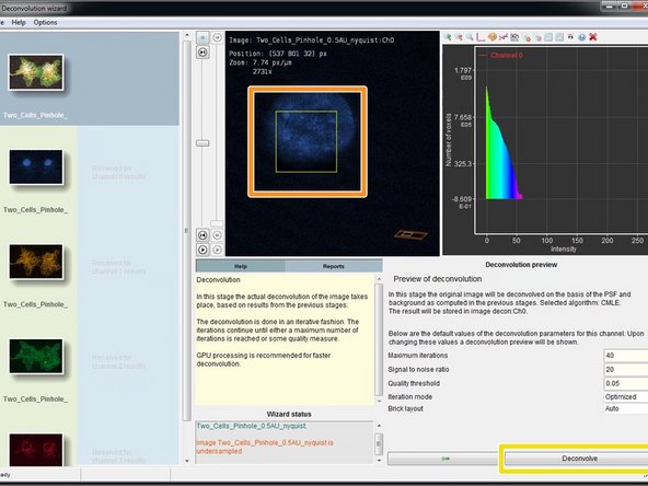
To check the choosen deconvolution parameters you can click on "Deconvolution preview".

In the image window you can see now a yellow box which previews the result of the deconvolution. If you are not happy or start seeing artifacts, you might need to adjust the deconvolution parameters such as the SNR.

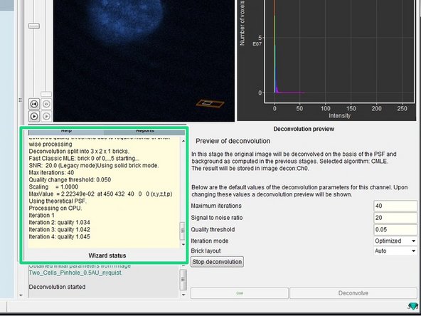
If the preview looks good, you can click "Deconvolve" which starts the deconvolution of the active channel.

The progress of your deconvolution can be seen in the "Reports" window. Keep in mind that deconvolving a dataset might take some time.

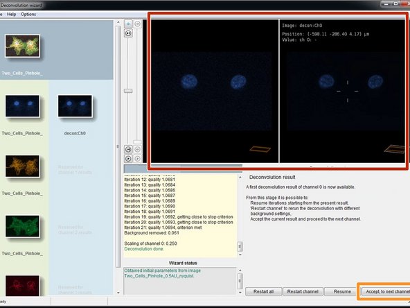
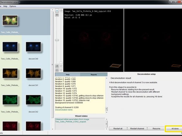
When the deconvolution of your channel is done, you can see a preview of the result in the "Deconvolution result" step.

Click "Accept, to next channel" to deconvolve the next channel of your dataset.

For the next channel, the wizard starts again on Step #12.

Perform a deconvolution for all channels of your dataset.

After deconvolution of the last channel click "All done".

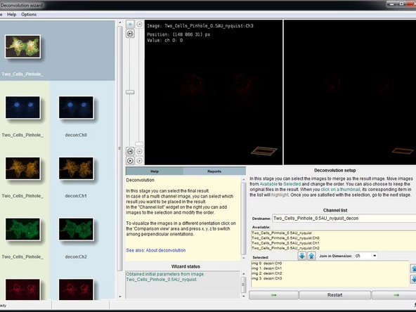
In this step you can select and merge the resulting channels. Usually nothing needs to be done here and you can click "next".

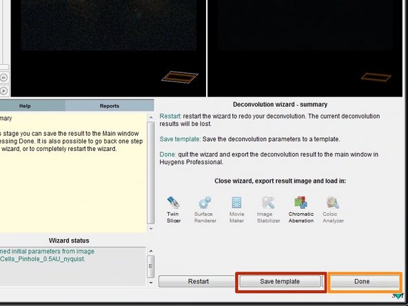
In the last step you can save your deconvolution parameters as a template. This can be useful if you deconvolve multiple datasets of the same type.

Click "Done" to close the deconvolution wizard.

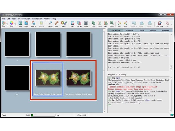
Back on the Huygens workspace you will find a new thumbnail with your deconvolution results.

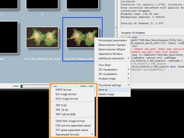
Save your results by right clicking on the results thumbnail and "Save as/...".

Usually saving your results as .tif is a good choice.

A "Question" dialog asks you how you want to save your files. Usually "One per channel and slice" is recommended.

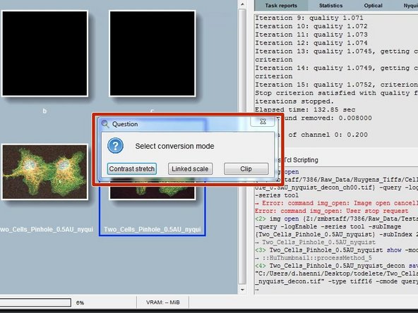
Depending on the choosen file format and the intensities in your data, Huygens might also ask about the conversion mode.

Contrast stretch: positive data range for each channel is adapted to the Tiff range, the different per-channel factors are not reported.

Linked scale: as stretch, but now the relation between channels is retained: the same factor is applied to all channels that stretches the one with maximum intensity to the Tiff range. The factor is reported by Huygens.

Clip: positive data outside the Tiff range is clipped to that range.

If the data is solely used for visualization purposes, "Contrast stretch" can be a good option. If ratiometric analysis of images is needed, then "Linked scale" might be the better option.

Please also read this article if you are unsure about what to choose here.

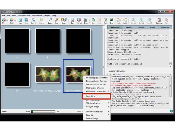
Finally, right click on the thumbnail and click "Twin Slicer".

In the drop down menu you can select your raw dataset on the left and your deconvolved dataset on the right for direct comparison of the deconvolution result.

If you are done with your deconvolution please save your data and close Huygens. Due to the license model we have with SVI we pay by usage. So idle Huygens session do cost us money. Thanks and good deconvolutions!